Rosenstiel School of Marine, Atmospheric, and Earth Science and Institute for Data Science and Computing
Last week you were asked:
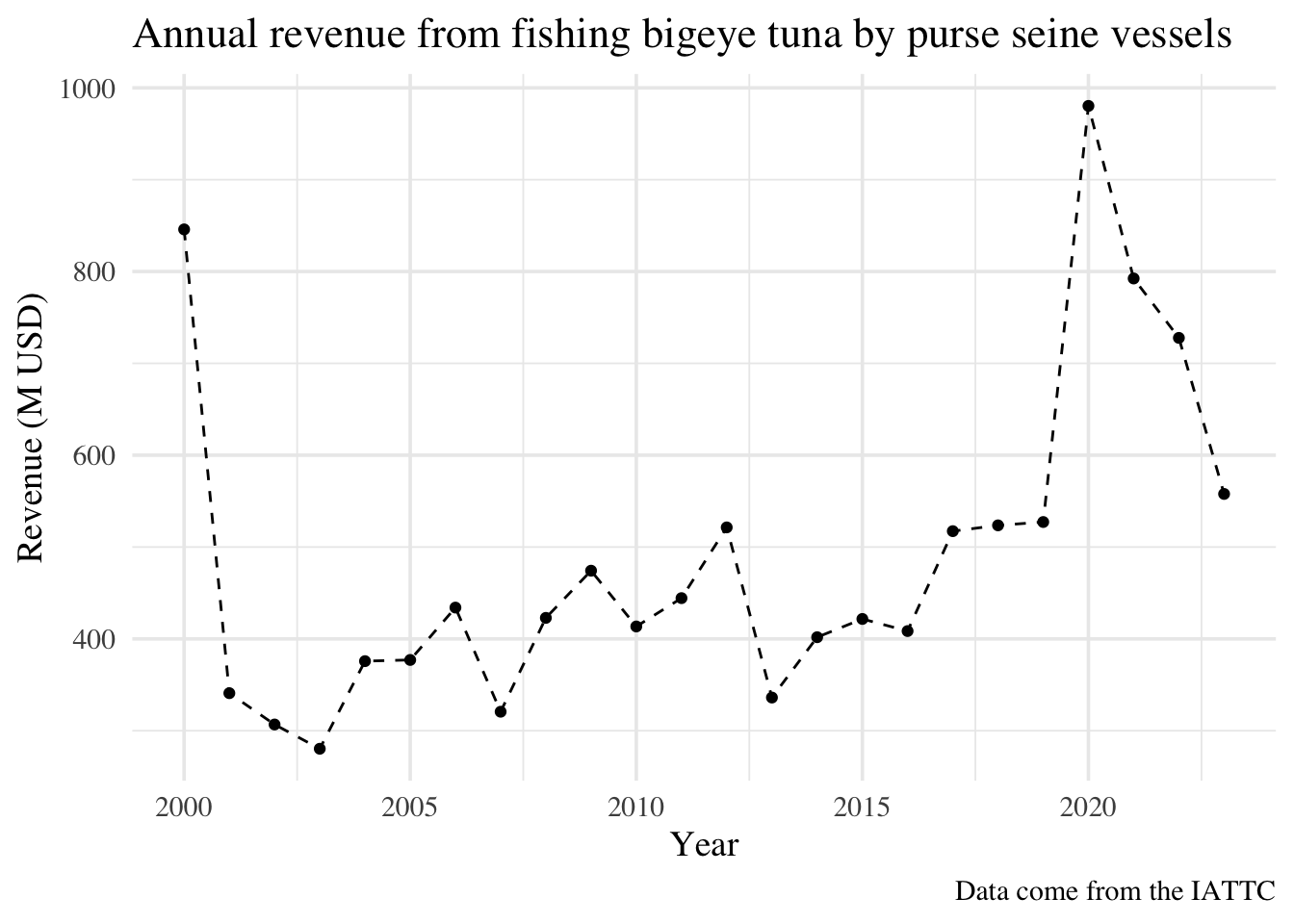
How much money have tuna purse seiners made since 2000 when fishing for bigeye tuna (Thunnus obesus) in the Eastern Pacific Ocean?
We made some simplifying assumptions and got some values (a total of 3,070 M USD since 2000, or about 127 M USD per year). You are now tasked with coming up with more refined estimates. For example, we will account for the fact that the price of fish varies every year.
How we will approach this:
Find data that shows prices per year and species
Read them, clean them, tidy them up (The “data tidying” part)
Combine our catch data from last week with this new price data (The “merging” part)
Re-calculate our total revenues since 2000
This will require three pipelines:
Tidy price data (Exercise 1)
Wrangle catch data (Exercise 2)
Combine tidy prices and catch data (Exercise 3)
Pipelines 1 and 3 contain tools covered this week. You should already be familiar with pipeline 2.
Exercise 1: Tidying price data
Part A: Downloading the data
Post-it up
In a web browser, go to ffa.int. This is the website for the Pacific Islands Forum Fisheries Agency
Hover over “Publication and Statistics” on the top menu
Select “Statistics”
You will be taken to a site with five items. Download the zip folder called Economic and Development Indicators and Statistics: Tuna Fishery of the Western and Central Pacific Ocean 2024
As before, place the downloaded zip file in your EVR628/data/raw folder and proceed to extract it
Open the excel file called Compendium of Economic and Development Statistics 2024 and study the Contents tab
Can you identify the price data that we need?
Which sheet
What range?
Post-it down
Part B: Reading excel data
Post-it up
Open your RStudio project for EVR628
In your console, install the readxl package: install.packages("readxl")
We will need three packages: readxl, janitor, and tidyverse, load them at the top of your script using library()
Use ?read_excel() to look at the documentation for the function
Use read_excel() to create a new object called tuna_prices and read the price data we need2. Immediately pipe it into clean_names.
Post-it down
Code
library(readxl)library(janitor)library(tidyverse)tuna_prices <-read_excel(path ="data/raw/Economic-and-Development-Indicators-and-Statistics-Tuna-Fishery-of-the-Western-and-Central-Pacific-Ocean-2024-32765/Compendium of Economic and Development Statistics 2024.xlsx",sheet ="B. Prices",range ="A35:E63",na ="na") |>clean_names()
Part C: Inspecting price data
Be prepared to discuss the following points:
Post-it up
Inspect the column names of tuna_prices using colnames() in your console.
How many columns and rows do we have?
Any missing values?
Do we need to make the data wider or longer?
Using comments, write out what the target data should be (expand my code chunk see what I wrote)
# A tibble: 4 × 5
   year japan_fresha japan_frozenb us_freshc us_frozend
  <dbl>        <dbl>         <dbl>     <dbl>      <dbl>
1  1997        8204.         8169.        NA         NA
2  1998        7703.         6320.        NA         NA
3  1999        8809.         9093.        NA         NA
4  2000        9198.         8557.        NA         NA
Code
# The final data set should have two columns: year and price. Since we have four# prices (two markets, two presentations), I will use the average price per year.# The tidy data set should therefore have four columns: year, market,# presentation, and price.
Part D: Tidy your price data
Post-it up
Look at the documentation for your pivot_* function. What does it say about cases where names_to is of length > 1?
What about the names_sep argument?
Use the appropriate pivot_* function to reshape your data and save them to a new object called tidy_tuna_prices3
Your resulting tibble should have 104 rows and 4 columns and look like this:4
# A tibble: 104 × 4
    year market presentation price
   <dbl> <chr>  <chr>        <dbl>
 1  1997 japan  fresha       8204.
 2  1997 japan  frozenb      8169.
 3  1998 japan  fresha       7703.
 4  1998 japan  frozenb      6320.
 5  1999 japan  fresha       8809.
 6  1999 japan  frozenb      9093.
 7  2000 japan  fresha       9198.
 8  2000 japan  frozenb      8557.
 9  2001 japan  fresha       8260.
10  2001 japan  frozenb      5983.
# ℹ 94 more rows
Post-it down
Values in presentation
Note that the values in the presentation column are not ideal. They end in a, b, c, and d due to footnotes included in Excel. For now this doesn’t matter because we will quickly remove them. We’ll cover some text wrangling in Week 9.
Part E: Calculate mean annual price
Post-it up
Modify the pipeline that creates tidy_tuna_prices to get the mean price per year5
Note: You can copy-paste and modify your code from last week, but make sure your code is organized.
Post-it up
Read in the tuna catch data from last week
Filter it to retain bigeye tuna (BET) caught by the purse seine fleet (PS) since 2000
Calculate total catch by year. Your final data should have 24 rows and 2 columns, as below
Post-it down
Code
# Load the datatuna_data <-read_csv("data/raw/CatchByFlagGear/CatchByFlagGear1918-2023.csv") |># Clean column namesclean_names() |># Rename some columnsrename(year = ano_year,flag = bandera_flag,gear = arte_gear,species = especies_species,catch = t)ps_tuna_data <- tuna_data |>filter(species =="BET", # Retain BET values only gear =="PS", # Retain PS values only year >=2000) |># Retain data from 2000group_by(year) |># Specify that I am grouping by year# Tell summarize that I want to collapse the catch column by summing all its valuessummarize(catch =sum(catch))ps_tuna_data
How do these plot and numbers compare to what we found last week?
Code
sum(tuna_revenues$revenue)
[1] 11752.32
Code
mean(tuna_revenues$revenue)
[1] 489.68
Code
# Build plotggplot(data = tuna_revenues, # Specify my datamapping =aes(x = year, y = revenue)) +# And my aestheticsgeom_line(linetype ="dashed") +# Add a dashed linegeom_point() +# With points on toplabs(x ="Year", # Add some labelsy ="Revenue (M USD)",title ="Annual revenue from fishing bigeye tuna by purse seine vessels",caption ="Data come from the IATTC") +# Modify the themetheme_minimal(base_size =14, # Font size 14base_family ="Times") # Font family Times
Extra exercises for you to practice
The following four exercises use data that are built directly in R. You will need to copy and paste the provided code in your console (or R script) to make sure the objects appear in your environment.
Exercise 1: Pivot Longer Practice
Scenario: You are a TA and have been given grade data where each row represents a student and columns represent their scores on assignments 1-4. You need to calculate the mean grade for each student.6
student_scores_long <- student_scores |>pivot_longer(cols =starts_with("assignment"), # All columns from assignment_1 to assignment_4names_to ="assignment", # Create new column called "assignment" with column namesvalues_to ="score") # Create new column called "score" with the valuesstudent_means <- student_scores_long |>group_by(student_id) |># Group rows by student_idsummarize(mean_grade =mean(score)) # Calculate mean score for each studentstudent_means # View the result
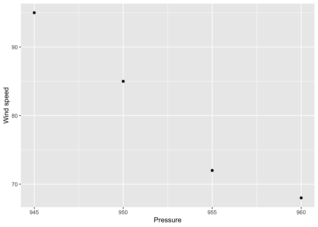
Scenario: You have hurricane exposure data from different Florida counties. You are asked to build a figure showing the relationship between pressure and wind speed. Modify the data as needed and build a figure.7
hurricane_wide <- hurricane_data |>pivot_wider(names_from = metric, # Use values in "metric" column as new column namesvalues_from = measurement) # Use values in "measurement" column to fill new columnshurricane_wide # Now each county is a row with separate columns for pressure, precipitation, wind_speed
Scenario: You have two datasets - one with student information and another with their enrollment details. You need to be able to identify the names of students taking stats courses.
# A tibble: 5 × 3
  student_id name            age
  <chr>      <chr>         <dbl>
1 S001       Alice Johnson    20
2 S002       Bob Smith        22
3 S003       Carol Davis      19
4 S004       David Wilson     21
5 S005       Eva Brown        23
combined_data <- students |>left_join(enrollments, by =join_by(student_id == stdt_identifier)) # Keep all students, match different column namescombined_data # View the combined data
# A tibble: 7 × 5
  student_id name            age course     credits
  <chr>      <chr>         <dbl> <chr>        <dbl>
1 S001       Alice Johnson    20 Statistics       3
2 S001       Alice Johnson    20 Biology          4
3 S002       Bob Smith        22 Statistics       3
4 S003       Carol Davis      19 Chemistry        4
5 S004       David Wilson     21 Statistics       3
6 S004       David Wilson     21 Physics          4
7 S005       Eva Brown        23 <NA>            NA
Code
statistics_students <- combined_data |>filter(course =="Statistics") |># Keep only rows where course equals "Statistics"select(name, course) # Keep only the name and course columnsstatistics_students # View the result
# A tibble: 3 × 2
  name          course
  <chr>         <chr>
1 Alice Johnson Statistics
2 Bob Smith     Statistics
3 David Wilson  Statistics
Exercise 4: Sharks!
Scenario: You have swimming data from beachgoers and bull shark detection data from acoustic telemetry during fourth of July. The swimming data tell you when someone entered and left the water. The shark detection data tells you which sharks were detected within the acoustic array in front of the beach, and the time of detection. Who was in the water while a shark was nearby?8
swimmer_shark_overlap <- shark_detections |>inner_join(swimming_data, # Note that I am using an inner join. Play with inner, left, and right to see what happensby =join_by(between(detection_time, swim_start, swim_end))) # Find swimmers in water during shark detectionsswimmer_shark_overlap # View all the overlap data
# A tibble: 5 × 5
  shark_id detection_time      name  swim_start          swim_end
  <chr>    <dttm>              <chr> <dttm>              <dttm>
1 SH002    2024-07-04 11:25:00 Bob   2024-07-04 10:45:00 2024-07-04 11:30:00
2 SH002    2024-07-04 11:25:00 Carol 2024-07-04 11:00:00 2024-07-04 11:45:00
3 SH002    2024-07-04 11:25:00 David 2024-07-04 11:20:00 2024-07-04 12:00:00
4 SH003    2024-07-04 11:35:00 Carol 2024-07-04 11:00:00 2024-07-04 11:45:00
5 SH003    2024-07-04 11:35:00 David 2024-07-04 11:20:00 2024-07-04 12:00:00
Code
at_risk_swimmers <- swimmer_shark_overlap |>group_by(name) |># Keep only the columns we want to seesummarize(n_sharks_near =n_distinct(shark_id))at_risk_swimmers # These swimmers were in the water when sharks were detected
# A tibble: 3 × 2
  name  n_sharks_near
  <chr>         <int>
1 Bob               1
2 Carol             2
3 David             2
Footnotes
I would typically suggest to overwrite whatever we had last week in tuna_analysis.R because GitHub would keep a version, but I understand you might want to keep the script as is↩︎
Hint: You will need to specify a file path, a sheet, and a range of cells.↩︎
Hint: Your names_to argument should be a character vector of with two items. names_ _sep should be inspired by our clever use of snake_case.↩︎
Hint: If you have 112 rows, remember you can use values_drop_na = T↩︎
Hint: You will use group_by() and summarize(), as well as |>↩︎
Hint: Use pivot_longer() to transform this data so that each row represents one student-assignment-score combination, then use group_by() and summarize() to calculate the mean grade for each student.↩︎
Hint: Use pivot_wider() to transform this data so that each row represents a county and each metric becomes its own column.↩︎
Hint: Look at the documentation for join_by(). What does it say about “Overlap helpers”? You’ll want to use the between() function.↩︎