EVR 628- Intro to Environmental Data Science

Data Management and Transformation

Juan Carlos Villaseñor-Derbez (JC)

Learning Objectives

By the end of this week, you should be able to:

Know the difference between absolute and relative file paths
Read and write tabular data (*.xlsx, *.csv and *.rds)
Modify rows
Modify columns
Group and summarize data

Today’s Class

File paths and working directories
Reading and writing data
Data transformation with {dplyr}
- Row operations: filter()
- Column operations: select(), rename(), and mutate()
- Table operations: group_by() and summarize()

File Paths and Working Directories

Understanding File Paths

Important concepts

File path: The location of a file on your computer
Working directory: The folder R considers as “home” for your current session. It is given by the location of the .Rproj file.

Two types of paths:

Absolute path: Complete address from your hard drive as the origin
- Example: /Users/jcvd/GitHub/EVR_628/data/raw/dive_profile.csv
Relative path: Address relative to your current working directory
- Example: data/raw/dive_profile.csv

Understanding File Paths

Think of a file path as an address.

You can specify the full address (absolute path):
- USA/FL/Miami/Rickenbacker Causeway/Rosenstiel School/SLAB/Room 120
But if we all know Rosenstiel is the origin, we can use a relative address:
- SLAB/Room 120

Relative paths are best because they work across computers

Important

Best Practice: Use RStudio projects instead of setwd()

RStudio Projects and File Paths

Why projects are better:

Working directory is automatically set
Relative paths work consistently
Easy to share and reproduce
No need to remember absolute paths

If we are in my EVR628 RProject:

# Both work in my computer, only one will work in yours:
my_dive <- read.csv("/Users/jcvd/GitHub/EVR628/data/raw/dive_profile.csv") # Absolute
my_dive <- read.csv("data/raw/dive_profile.csv") # Relative

Reading and Writing Data

Three Relevant Data File Types

Focus on reading plain-text rectangular files

CSV Files

.csv format
Comma-separated values
Human-readable (ish)
Probably the most common format
Can be read into Excel in a pinch

Excel Files

.xlsx format
Common in business
Can have multiple sheets
Preserves formatting (irrelevant)

RDS Files

R’s native format
Preserves data types (characters, factors)
Compressed
Fastest to read/write in a computer
Not human readable

Reading CSV Files

CSV files can be human readable:

AnoYear,BanderaFlag,ArteGear,EspeciesSpecies,t
1918,UNK,LP,SKJ,1361
1918,UNK,LP,YFT,0
1919,UNK,LP,SKJ,3130
1919,UNK,LP,YFT,136
1920,UNK,LP,SKJ,3583
1920,UNK,LP,YFT,907
1921,UNK,LP,SKJ,499
1921,UNK,LP,YFT,590
1922,UNK,LP,SKJ,5398

The first row has the “header”, containing the column names
Commas “,” indicate the separation between columns

Reading CSV files is straightforward:

library(tidyverse) # We need the tidyverse

tuna_data <- read_csv(file = "data/raw/CatchByFlagGear1918-2023.csv") # Simply specify the filepath

Similar formats are tsv and txt

Reading Excel Files

Reading excel files is also straighforward, but requires additional packages

# Install if needed
# install.packages("readxl")

# Load package
library(readxl)

# Read first sheet
data <- read_excel(path = "data/raw/lionfish.xlsx",
                   sheet = 2,
                   range = "A1:B20")

I don’t recommend using Excel to store your raw data.
Excel likes to modify strings that might look like dates:
- 25% of papers on human Genes had gene names converted to dates by Excel
- See Ziemann, Eren, and El-Osta (2016) for details
There are a few alternatives:
- Use a CSV editor
- Use a data entry platform that exports data as csv (or similar)

Reading RDS Files

Reading RDS files is just as easy:

# Using readr
data <- read_rds(file = "data/raw/lionfish.rds")

A Recommended Workflow

I receive data either in xls or csv
Read the data as needed
Modify / clean / filter / wrangle
Export processed data as .rds

Writing Data Files

We used read_* to read data…

And yes, we use write_* to write data

# Write RDS
write_rds(x = clean_tuna_data, file = "data/processed/tuna_clean.rds")

# Write CSV with readr
write_csv(x = clean_tuna_data, file = "data/processed/tuna_clean.csv")

Example: Working with Real Data

On Thursday we will work with public domain data from the IATTC
Specifically, data on EPO total estimated catch by year, flag, gear, species (1918 - 2023)
But the data are a bit messy!
Today is when we start to learn about data wrangling with two key packages:
- {dplyr}(part of the tidyverse, no need to install it)
- {janitor}

Data transformation with `{dplyr}`

Common Data Transformations

Filter data
Rename variables
Arrange the order in which variables appear
Create new variables
Summarize information in a variable, often across groups
Arrange the order in which observations appear

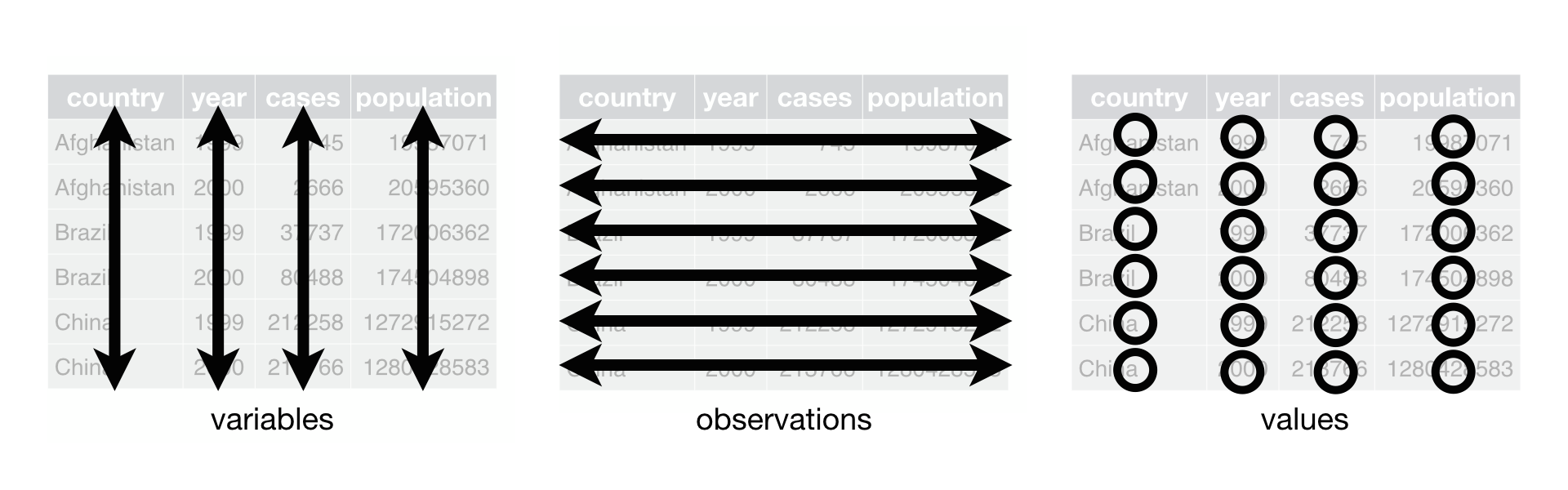
On Tidy Data

The dplyr package, like ggplot2 relies on data being in this format:

Columns are variables
Rows are observations
Cells contain values

Image Credit: Wickham, Mine Cetinkaya-Rundel, and Grolemund (2023)

The `{dplyr}` Package

{dplyr}: A grammar of data manipulation

Core functions:

filter(): Pick observations by their values
select(): Pick variables by their names
mutate(): Create new variables with functions of existing variables
group_by(): Change the scope of each function from operating on the entire dataset to operating on it group-by-group
summarize(): Collapse many values down to a single summary

Common Features of `dplyr` functions

First argument is always a data.frame or tibble
The arguments that follow specify which columns we are working on
dplyr functions always return a new data.frame
This class(input) == class(output) condition means we can easily build pipelines

dplyr functions are also referred to as dplyr verbs, because they all imply an action

dplyr verbs are organized into four groups based on what they operate on: rows, columns, or groups

Row operations

filter()

Recall the `data_MPA` data

data_MPA

# A tibble: 100 × 5
    time id    protected after biomass
   <int> <chr>     <dbl> <dbl>   <dbl>
 1    -5 a             1     0    9.37
 2    -5 b             1     0   10.2 
 3    -5 c             1     0    9.16
 4    -5 d             1     0   11.6 
 5    -5 e             1     0   10.3 
 6    -5 f             0     0    9.18
 7    -5 g             0     0   10.5 
 8    -5 h             0     0   10.7 
 9    -5 i             0     0   10.6 
10    -5 j             0     0    9.69
# ℹ 90 more rows

Filtering Rows with `filter()`

filter(): Keep rows that match your conditions

Example: Keep data from protected sites

# Shorthand syntax
#     (data,  Condition)
filter(data_MPA, protected == 1)

# A tibble: 50 × 5
    time id    protected after biomass
   <int> <chr>     <dbl> <dbl>   <dbl>
 1    -5 a             1     0    9.37
 2    -5 b             1     0   10.2 
 3    -5 c             1     0    9.16
 4    -5 d             1     0   11.6 
 5    -5 e             1     0   10.3 
 6    -4 a             1     0   11.5 
 7    -4 b             1     0   10.4 
 8    -4 c             1     0    9.38
 9    -4 d             1     0    7.79
10    -4 e             1     0   11.1 
# ℹ 40 more rows

# Full syntax
filter(.data = data_MPA, protected == 1)
# Tidy syntax
data_MPA |> 
  filter(protected == 1)

Filtering Rows with `filter()`

Multiple conditions require using logical operators

Example: All data from sites “a” and “b”, after the MPA was established

data_MPA |> 
    filter((id == "a" | id == "b"), # Keep data where id is equal to a or b AND
           after == 1) # where after is equals to 1

# A tibble: 10 × 5
    time id    protected after biomass
   <int> <chr>     <dbl> <dbl>   <dbl>
 1     0 a             1     1    12.4
 2     0 b             1     1    11.4
 3     1 a             1     1    14.4
 4     1 b             1     1    12.0
 5     2 a             1     1    12.5
 6     2 b             1     1    11.3
 7     3 a             1     1    11.4
 8     3 b             1     1    11.9
 9     4 a             1     1    11.5
10     4 b             1     1    13.2

Filtering Rows with `filter()`

You can leverage the “%in%” operator to avoid typing too much

Example: All data from sites “a”, “b”, “c”, and “d”, on the first year

data_MPA |> 
    filter(id %in% c("a", "b", "c", "d"),
           time == min(time))

# A tibble: 4 × 5
   time id    protected after biomass
  <int> <chr>     <dbl> <dbl>   <dbl>
1    -5 a             1     0    9.37
2    -5 b             1     0   10.2 
3    -5 c             1     0    9.16
4    -5 d             1     0   11.6

Column operations

select(), rename(), and mutate()

Back to `data_lionfish`

data_lionfish

# A tibble: 109 × 9
   id       site    lat   lon total_length_mm total_weight_gr size_class depth_m
   <chr>    <chr> <dbl> <dbl>           <dbl>           <dbl> <chr>        <dbl>
 1 001-Po-… Para…  20.5 -87.2             213           113.  large         38.1
 2 002-Po-… Para…  20.5 -87.2             124            27.6 medium        27.9
 3 003-Pd-… Pared  20.5 -87.2             166            52.3 medium        18.5
 4 004-Cs-… Cano…  20.5 -87.2             203           123.  large         15.5
 5 005-Cs-… Cano…  20.5 -87.2             212           129   large         15  
 6 006-Pl-… Paam…  20.5 -87.2             210           139.  large         22.7
 7 007-Pl-… Paam…  20.5 -87.2             132            50.3 medium        13.4
 8 008-Po-… Para…  20.5 -87.2             122            17.2 medium        18.5
 9 009-Po-… Para…  20.5 -87.2             224           113.  large         18.2
10 010-Pd-… Pared  20.5 -87.2             117            19.6 medium        12.5
# ℹ 99 more rows
# ℹ 1 more variable: temperature_C <dbl>

1) Selecting Columns with `select()`

select(): Allows us to state which columns we want to keep

Select columns by name

# Select specific columns
data_lionfish |> 
  select(id, total_length_mm, total_weight_gr)

# A tibble: 109 × 3
   id              total_length_mm total_weight_gr
   <chr>                     <dbl>           <dbl>
 1 001-Po-16/05/10             213           113. 
 2 002-Po-29/05/10             124            27.6
 3 003-Pd-29/05/10             166            52.3
 4 004-Cs-12/06/10             203           123. 
 5 005-Cs-12/06/10             212           129  
 6 006-Pl-21/06/10             210           139. 
 7 007-Pl-21/06/10             132            50.3
 8 008-Po-04/07/10             122            17.2
 9 009-Po-04/07/10             224           113. 
10 010-Pd-08/07/10             117            19.6
# ℹ 99 more rows

Select columns by position

# Select columns by position
data_lionfish |> 
  select(c(1, 5:6))

# A tibble: 109 × 3
   id              total_length_mm total_weight_gr
   <chr>                     <dbl>           <dbl>
 1 001-Po-16/05/10             213           113. 
 2 002-Po-29/05/10             124            27.6
 3 003-Pd-29/05/10             166            52.3
 4 004-Cs-12/06/10             203           123. 
 5 005-Cs-12/06/10             212           129  
 6 006-Pl-21/06/10             210           139. 
 7 007-Pl-21/06/10             132            50.3
 8 008-Po-04/07/10             122            17.2
 9 009-Po-04/07/10             224           113. 
10 010-Pd-08/07/10             117            19.6
# ℹ 99 more rows

1) Selecting Columns with `select()`

Select columns by partial name match

# Select columns by pattern
select(data_lionfish, contains("total"))

# A tibble: 109 × 2
   total_length_mm total_weight_gr
             <dbl>           <dbl>
 1             213           113. 
 2             124            27.6
 3             166            52.3
 4             203           123. 
 5             212           129  
 6             210           139. 
 7             132            50.3
 8             122            17.2
 9             224           113. 
10             117            19.6
# ℹ 99 more rows

Remove columns by position

# Exclude columns
select(data_lionfish, -c(6:9))

# A tibble: 109 × 5
   id              site      lat   lon total_length_mm
   <chr>           <chr>   <dbl> <dbl>           <dbl>
 1 001-Po-16/05/10 Paraiso  20.5 -87.2             213
 2 002-Po-29/05/10 Paraiso  20.5 -87.2             124
 3 003-Pd-29/05/10 Pared    20.5 -87.2             166
 4 004-Cs-12/06/10 Canones  20.5 -87.2             203
 5 005-Cs-12/06/10 Canones  20.5 -87.2             212
 6 006-Pl-21/06/10 Paamul   20.5 -87.2             210
 7 007-Pl-21/06/10 Paamul   20.5 -87.2             132
 8 008-Po-04/07/10 Paraiso  20.5 -87.2             122
 9 009-Po-04/07/10 Paraiso  20.5 -87.2             224
10 010-Pd-08/07/10 Pared    20.5 -87.2             117
# ℹ 99 more rows

Helper Functions for `select()`

Selection helpers:

contains(): Contains substring
starts_with(): Starts with prefix
ends_with(): Ends with suffix
everything(): All other columns columns

2) Renaming Columns with `rename()`

rename(): Change column names

Example: Rename id to fish_id, total_length_mm to length_mm, and total_weight_mm to weight_gr

# Rename specific columns
rename(data_lionfish,
       fish_id = id,
       length = total_length_mm,
       weight = total_weight_gr)

# A tibble: 109 × 9
   fish_id      site    lat   lon length weight size_class depth_m temperature_C
   <chr>        <chr> <dbl> <dbl>  <dbl>  <dbl> <chr>        <dbl>         <dbl>
 1 001-Po-16/0… Para…  20.5 -87.2    213  113.  large         38.1            28
 2 002-Po-29/0… Para…  20.5 -87.2    124   27.6 medium        27.9            28
 3 003-Pd-29/0… Pared  20.5 -87.2    166   52.3 medium        18.5            28
 4 004-Cs-12/0… Cano…  20.5 -87.2    203  123.  large         15.5            28
 5 005-Cs-12/0… Cano…  20.5 -87.2    212  129   large         15              28
 6 006-Pl-21/0… Paam…  20.5 -87.2    210  139.  large         22.7            29
 7 007-Pl-21/0… Paam…  20.5 -87.2    132   50.3 medium        13.4            29
 8 008-Po-04/0… Para…  20.5 -87.2    122   17.2 medium        18.5            29
 9 009-Po-04/0… Para…  20.5 -87.2    224  113.  large         18.2            29
10 010-Pd-08/0… Pared  20.5 -87.2    117   19.6 medium        12.5            29
# ℹ 99 more rows

Note that the syntax is new_name = old_name

3) Creating New Columns with `mutate()`

mutate(): Add new columns or modify existing ones

# Create new columns
data_lionfish |> 
  mutate(length_weight_ratio = total_length_mm / total_weight_gr)

# A tibble: 109 × 10
   id       site    lat   lon total_length_mm total_weight_gr size_class depth_m
   <chr>    <chr> <dbl> <dbl>           <dbl>           <dbl> <chr>        <dbl>
 1 001-Po-… Para…  20.5 -87.2             213           113.  large         38.1
 2 002-Po-… Para…  20.5 -87.2             124            27.6 medium        27.9
 3 003-Pd-… Pared  20.5 -87.2             166            52.3 medium        18.5
 4 004-Cs-… Cano…  20.5 -87.2             203           123.  large         15.5
 5 005-Cs-… Cano…  20.5 -87.2             212           129   large         15  
 6 006-Pl-… Paam…  20.5 -87.2             210           139.  large         22.7
 7 007-Pl-… Paam…  20.5 -87.2             132            50.3 medium        13.4
 8 008-Po-… Para…  20.5 -87.2             122            17.2 medium        18.5
 9 009-Po-… Para…  20.5 -87.2             224           113.  large         18.2
10 010-Pd-… Pared  20.5 -87.2             117            19.6 medium        12.5
# ℹ 99 more rows
# ℹ 2 more variables: temperature_C <dbl>, length_weight_ratio <dbl>

3) Recreating Columns with `mutate()`

You can overwrite an existing column

You can use conditional logic

# Using case_when()
data_lionfish |> 
  mutate(size_class = ifelse(total_length_mm < 150, "small", "large"))

# A tibble: 109 × 9
   id       site    lat   lon total_length_mm total_weight_gr size_class depth_m
   <chr>    <chr> <dbl> <dbl>           <dbl>           <dbl> <chr>        <dbl>
 1 001-Po-… Para…  20.5 -87.2             213           113.  large         38.1
 2 002-Po-… Para…  20.5 -87.2             124            27.6 small         27.9
 3 003-Pd-… Pared  20.5 -87.2             166            52.3 large         18.5
 4 004-Cs-… Cano…  20.5 -87.2             203           123.  large         15.5
 5 005-Cs-… Cano…  20.5 -87.2             212           129   large         15  
 6 006-Pl-… Paam…  20.5 -87.2             210           139.  large         22.7
 7 007-Pl-… Paam…  20.5 -87.2             132            50.3 small         13.4
 8 008-Po-… Para…  20.5 -87.2             122            17.2 small         18.5
 9 009-Po-… Para…  20.5 -87.2             224           113.  large         18.2
10 010-Pd-… Pared  20.5 -87.2             117            19.6 small         12.5
# ℹ 99 more rows
# ℹ 1 more variable: temperature_C <dbl>

Grouping and summarizing

First, let’s modify the `data_MPA` object

Recall that it looked like this:

data_MPA

# A tibble: 100 × 5
    time id    protected after biomass
   <int> <chr>     <dbl> <dbl>   <dbl>
 1    -5 a             1     0    9.37
 2    -5 b             1     0   10.2 
 3    -5 c             1     0    9.16
 4    -5 d             1     0   11.6 
 5    -5 e             1     0   10.3 
 6    -5 f             0     0    9.18
 7    -5 g             0     0   10.5 
 8    -5 h             0     0   10.7 
 9    -5 i             0     0   10.6 
10    -5 j             0     0    9.69
# ℹ 90 more rows

I’d rather have it like this:

data_MPA <- data_MPA |> 
  mutate(protected = ifelse(protected == 1, "yes", "no"),
         after = ifelse(after == 1, "after", "before"))

data_MPA

# A tibble: 100 × 5
    time id    protected after  biomass
   <int> <chr> <chr>     <chr>    <dbl>
 1    -5 a     yes       before    9.37
 2    -5 b     yes       before   10.2 
 3    -5 c     yes       before    9.16
 4    -5 d     yes       before   11.6 
 5    -5 e     yes       before   10.3 
 6    -5 f     no        before    9.18
 7    -5 g     no        before   10.5 
 8    -5 h     no        before   10.7 
 9    -5 i     no        before   10.6 
10    -5 j     no        before    9.69
# ℹ 90 more rows

1) Grouping Data with `group_by()`

group_by(): Group data by one or more variables

# Group by protection status and timing
data_MPA |> 
  group_by(protected, after)

# A tibble: 100 × 5
# Groups:   protected, after [4]
    time id    protected after  biomass
   <int> <chr> <chr>     <chr>    <dbl>
 1    -5 a     yes       before    9.37
 2    -5 b     yes       before   10.2 
 3    -5 c     yes       before    9.16
 4    -5 d     yes       before   11.6 
 5    -5 e     yes       before   10.3 
 6    -5 f     no        before    9.18
 7    -5 g     no        before   10.5 
 8    -5 h     no        before   10.7 
 9    -5 i     no        before   10.6 
10    -5 j     no        before    9.69
# ℹ 90 more rows

This might not seem like much, until you hear about summarize()

2) Summarizing Data with `summarize()`

summarize(): Collapse groups to single values (and create a new column)

Example: Calculate mean biomass by protection site and study period

data_MPA |> 
  group_by(protected, after) |> # Define the groups
  summarize(biomass_m = mean(biomass)) # Collapse the biomass values of each group into a single value

# A tibble: 4 × 3
# Groups:   protected [2]
  protected after  biomass_m
  <chr>     <chr>      <dbl>
1 no        after       10.1
2 no        before      10.1
3 yes       after       12.2
4 yes       before      10.1

Common Summary Functions

Count functions:

n(): Number of observations
n_distinct(): Number of unique values

Summary functions:

stats: mean(), median(), sd(), min(), max()
positional: first(), last(), nth()

2) Summarizing Data with `summarize()`

You can calculate multiple summaries at once

Example: Let’s calculate the mean biomass and sd of biomass for each treatment status

# Summary by group
data_MPA |> 
  group_by(protected, after) |> 
  summarize(biomass_m = mean(biomass),
            biomass_sd = sd(biomass))

# A tibble: 4 × 4
# Groups:   protected [2]
  protected after  biomass_m biomass_sd
  <chr>     <chr>      <dbl>      <dbl>
1 no        after       10.1      0.953
2 no        before      10.1      0.648
3 yes       after       12.2      1.000
4 yes       before      10.1      0.995

On Thursday

Revisit the data_MPA analysis, this time with dplyr verbs
Walk you through downloading publicly available data
We will work with public domain data from the IATTC
Specifically, data on EPO total estimated catch by year, flag, gear, species (1918 - 2023)
Build a data cleaning pipeline
Export clean data

Learning Objectives - Revisited

By the end of this week, you should be able to:

Know the difference between absolute and relative file paths
Read and write tabular data (*.xlsx, *.csv and *.rds)
Modify rows (filter(), arrange())
Modify columns (select(), rename())
Group and summarize data

Let’s get coding

Go to jcvdav.github.io/EVR_628 and find the guide for live coding

References

Wickham, Hadley, Mine Cetinkaya-Rundel, and Garrett Grolemund. 2023. R for Data Science: Import, Tidy, Transform, Visualize, and Model Data. 2nd ed. Sebastopol, CA: O’Reilly Media.

Ziemann, Mark, Yotam Eren, and Assam El-Osta. 2016. “Gene Name Errors Are Widespread in the Scientific Literature.” Genome Biology 17 (1): 177.

EVR 628- Intro to Environmental Data Science

Learning Objectives

Today’s Class

File Paths and Working Directories

Understanding File Paths

Understanding File Paths

RStudio Projects and File Paths

Reading and Writing Data

Three Relevant Data File Types

Reading CSV Files

Reading Excel Files

Reading RDS Files

Writing Data Files

Example: Working with Real Data

Data transformation with {dplyr}

Common Data Transformations

On Tidy Data

The {dplyr} Package

Common Features of dplyr functions

Row operations

Recall the data_MPA data

Filtering Rows with filter()

Filtering Rows with filter()

Filtering Rows with filter()

Column operations

Back to data_lionfish

1) Selecting Columns with select()

1) Selecting Columns with select()

Helper Functions for select()

2) Renaming Columns with rename()

3) Creating New Columns with mutate()

3) Recreating Columns with mutate()

Grouping and summarizing

First, let’s modify the data_MPA object

1) Grouping Data with group_by()

2) Summarizing Data with summarize()

Common Summary Functions

2) Summarizing Data with summarize()

On Thursday

Learning Objectives - Revisited

Let’s get coding

References

Data transformation with `{dplyr}`

The `{dplyr}` Package

Common Features of `dplyr` functions

Recall the `data_MPA` data

Filtering Rows with `filter()`

Filtering Rows with `filter()`

Filtering Rows with `filter()`

Back to `data_lionfish`

1) Selecting Columns with `select()`

1) Selecting Columns with `select()`

Helper Functions for `select()`

2) Renaming Columns with `rename()`

3) Creating New Columns with `mutate()`

3) Recreating Columns with `mutate()`

First, let’s modify the `data_MPA` object

1) Grouping Data with `group_by()`

2) Summarizing Data with `summarize()`

2) Summarizing Data with `summarize()`