Coding Principles Exercises

EVR 628- Intro to Environmental Data Science

Author

Affiliation

Juan Carlos Villaseñor-Derbez (JC)

Rosenstiel School of Marine, Atmospheric & Earth Science and Institute for Data Science & Computing

Exercise 1: Object Classes and Assignment

Part A: Set up

1. Open R Studio and navigate to your EVR628 project
2. Set up a code snippet for a header

################################################################################
# title
################################################################################
#
# Your Name Here
# Your email here
# date
#
# Description
#
################################################################################

3. Create a new R script and save it as objects_and_classes.R
4. Use your new code snippet to add the header

Part B: Create and Check Object Classes

In your R Script, create objects of different classes and check their types:

1. A character object called my_name with your name
2. A numeric object called my_lucky_number with your lucky number (or any number, it doesn’t have to be your lucky number)
3. A logical object called is_student with TRUE or FALSE (note the all caps)
4. Check the class of each object using class()

my_name <- "JC" # character object called `my_name` with your name
my_lucky_number <- 32 # numeric object called `my_lucky_number` with your lucky number
is_student <- FALSE # logical object called `is_student` with TRUE or FALSE

# Check the class of each object using `class()`
class(my_name)

[1] "character"

class(my_lucky_number)

[1] "numeric"

class(is_student)

[1] "logical"

Part C: Object Coercion

Let’s see what happens when you try converting objects. In the R script, write and then execute code that will:

1. Convert your lucky number to character using as.character(my_lucky_number)
2. Convert TRUE to numeric using as.numeric()
3. Try to convert "hello" to numeric - what happens?
4. Advanced: Use |> to build a code pipeline to:
   1. Take your lucky number
   2. Convert it to character
   3. Get it’s class

# Note that I am overwriting the object. If I had only done
# `as.character(my_lucky_number)`, then the coerced output would have been
# printed to the console.
my_lucky_number <- as.character(my_lucky_number) # Convert your lucky number to `character`

# Check that it worked
class(my_lucky_number)

[1] "character"

as.numeric(TRUE) # Convert `TRUE` to numeric using `as.numeric()`

[1] 1

as.numeric("hello") # Try to convert `"hello"` to `numeric` - what happens?

Warning: NAs introduced by coercion

[1] NA

# Build a pipeline
my_lucky_number <- 32 # Start with my_lucky_number as numeric again

# And now build the pipeline
my_lucky_number |> 
  as.character() |> 
  class()

[1] "character"

Exercise 2: Vectors and Operations

Part A: Create and Manipulate Vectors

1. Clean you environment (use the broom icon)
2. Create a numeric vector called length_m with values: 6, 4.1, 2.8, 5.5, 3.9, 5.8
3. Create a character vector called shark_species with: Great White Shark, Lemon Shark, Bull Shark, Hammerhead Shark, Mako Shark, and Great White Shark (yes, white shark again)
4. How many variables do you have in your environment?
5. How many length observations do we have? Find the length of both vectors using length()
6. How many unique species do we have? (Hint, use |> to build a pipeline)
7. Calculate the mean length of all sharks using mean()
8. Find the maximum length using max()

# Q2
length_m <- c(6, 4.1, 2.8, 5.5, 3.9, 5.8) 
# Q3
shark_species <- c("Great White Shark", "Lemon Shark", "Bull Shark", 
                   "Hammerhead Shark", "Mako Shark", "Great White Shark")
# Q5
length(length_m)

[1] 6

# Q6
shark_species |> 
  unique() |> 
  length()

[1] 5

# Q7
mean(x = length_m)

[1] 4.683333

# Q8
max(length_m)

[1] 6

Important

• When passing arguments to functions, use = not <-
• When creating objects, use <- not =

Part B: Vector Operations and Indexing

1. Extract the first 3 shark species using indexing with [] and save them to an object called first_3
2. Extract shark species where maximum length is greater than 4 meters
3. Assuming the values in length_m and sharks_species are ordered so that they match each other, find the shark species that is the largest
4. Calculate the mean length for all great white sharks

# Q1
first_3 <- shark_species[1:3] # Extract values 1 through 3 and assign them
first_3 # See the values I assigned

[1] "Great White Shark" "Lemon Shark"       "Bull Shark"       

# Q2
shark_species[length_m > 4] #Extract shark species where maximum length is greater than 4 meters

[1] "Great White Shark" "Lemon Shark"       "Hammerhead Shark" 
[4] "Great White Shark"

# Q3
shark_species[length_m == max(length_m)]

[1] "Great White Shark"

# Q4 (Option 1, no pipes)
# Read as : "Calculate the mean of lengths where shark species matches Great White Shark
mean(length_m[shark_species == "Great White Shark"])

[1] 5.9

# Q4 (Option 2, with pipe)
length_m[shark_species == "Great White Shark"] |> # Read as: Extract lengths where name matches great white shark AND THEN ...
  mean() # Calculate the mean

[1] 5.9

---

Likely pause here

---

Exercise 3: Data Frames and Tibbles

Part A: Estimate the effect of a Marine Protected Area on Biomass

1. Start a new script called MPA_analysis, add a comment outline and then load the EVR628tools and tidyverse packages.

2. Load and inspect the new ?data_MPA

   1. What are the dimensions of the data?
   2. What are the column names?
   3. How many unique() sites are there?
   4. How many unique() years?
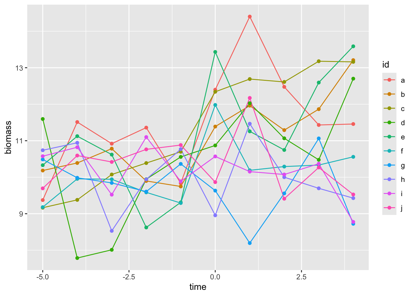
   5. Visualize the trends in biomass through time and across sites

3. Create four objects containing:

   1. Mean biomass inside the MPA before it was protected
   2. Mean biomass inside the MPA after it was protected
   3. Mean biomass outside the MPA before the MPA was created
   4. Mean biomass outside the MPA after the MPA was created

Hint: Use a combination of subsetting ([ ]), relational (==), and logical operators (&)

4. Then, calculate:

   1. Change after vs before for the protected site
   2. Change after vs before for the unprotected site

5. Finally, calculate the difference between these two values. This is called the naive difference-in-differences estimate. You are calculating the differences across treatments and across time. See Villasenor-Derbez et al. (2018) and Lynham and Villaseñor-Derbez (2024) for details.

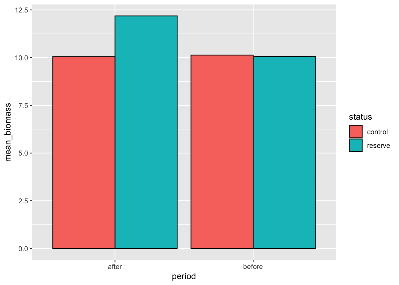
6. You now have four values, and you now where they come from. Assemble them into a new data.frame that allows you to build a figure where the x-axis is time, the y-axis is mean biomass, and colors are given by the protection status of the site.

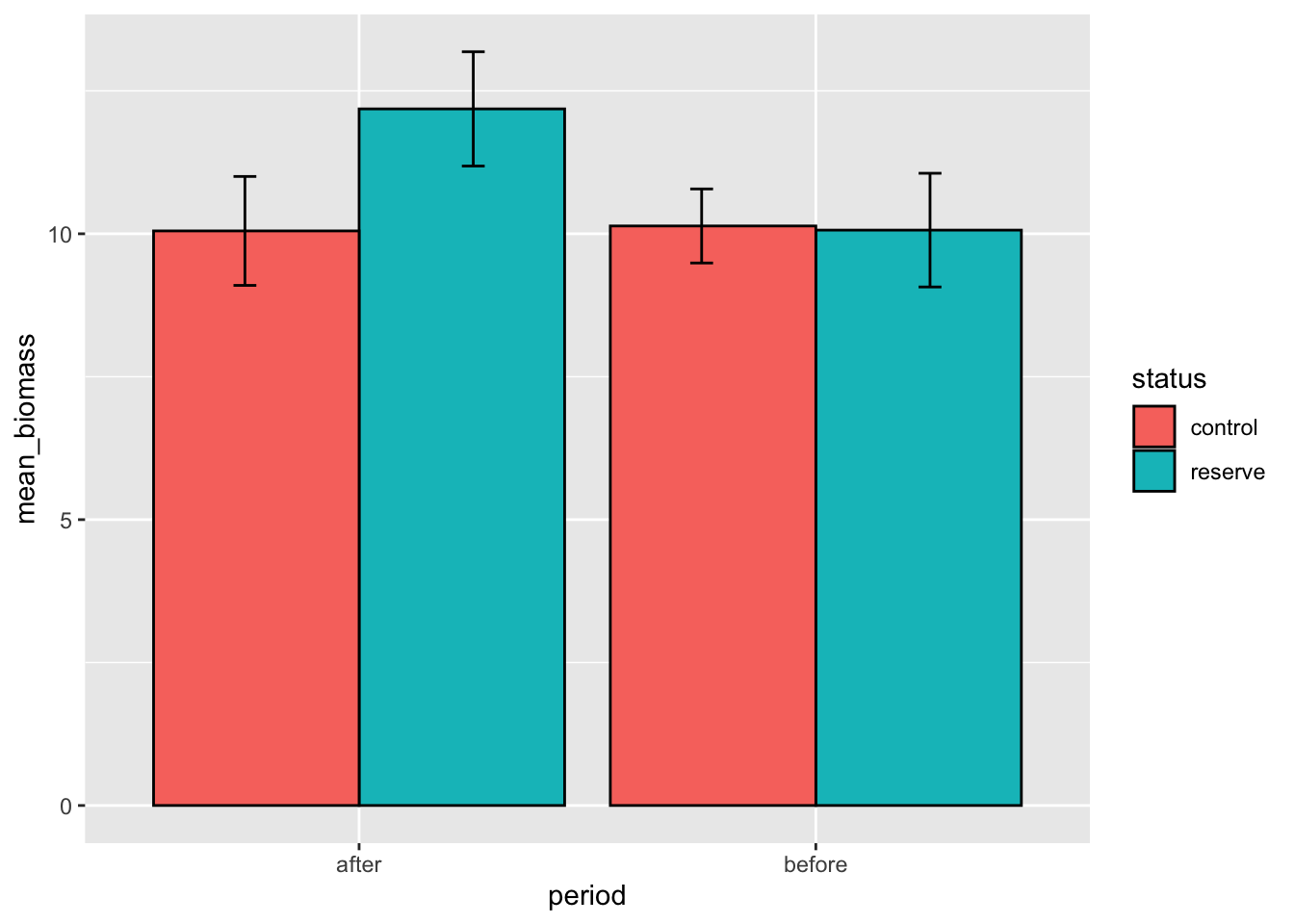
7. How would we go about adding standard deviations?

library(EVR628tools)
library(tidyverse)
data("data_MPA")

# 2e. Visualize
ggplot(data_MPA, aes(x = time, y = biomass, color = id)) + 
  geom_line() +
  geom_point()

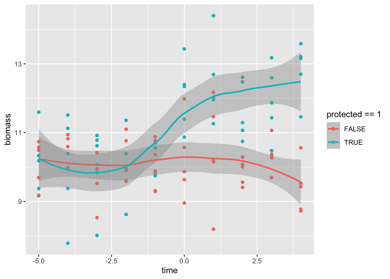
A better visualization:

ggplot(data_MPA, aes(x = time, y = biomass, color = protected == 1)) + 
  geom_point() +
  geom_smooth()

`geom_smooth()` using method = 'loess' and formula = 'y ~ x'

## Manually calculate DiD ------------------------------------------------------
# 3a.
mean_protected_before <- mean(data_MPA$biomass[data_MPA$protected == 1 & data_MPA$after == 0])

# 3b.
mean_protected_after <- mean(data_MPA$biomass[data_MPA$protected == 1 & data_MPA$after == 1])

# 3c.
mean_control_before <- mean(data_MPA$biomass[data_MPA$protected == 0 & data_MPA$after == 0])

# 3d.
mean_control_after <- mean(data_MPA$biomass[data_MPA$protected == 0 & data_MPA$after == 1])

# Difference in time for each site
# 4a.
dif_protected <- mean_protected_after - mean_protected_before

# 4b.
dif_control <- mean_control_after - mean_control_before

# Differences across sites
dif_in_dif <- dif_protected - dif_control

dif_in_dif

[1] 2.207114

# 6. Assemble the four values into a data.frame. Each vector I pass becomes a column,
# so I have to keep the order consistent across all three of them.
summary_data <- data.frame(period = c("before", "after", "before", "after"),
                           status = c("reserve", "reserve", "control", "control"),
                           mean_biomass = c(mean_protected_before,
                                            mean_protected_after,
                                            mean_control_before,
                                            mean_control_after))

summary_data

  period  status mean_biomass
1 before reserve     10.06411
2  after reserve     12.18455
3 before control     10.13678
4  after control     10.05011

# Now plot it
ggplot(summary_data, aes(x = period, y = mean_biomass, fill = status)) +
  geom_col(position = "dodge", color = "black")

# 7. Exactly the same subsetting as before, but with sd() instead of mean()
sd_protected_before <- sd(data_MPA$biomass[data_MPA$protected == 1 & data_MPA$after == 0])
sd_protected_after <- sd(data_MPA$biomass[data_MPA$protected == 1 & data_MPA$after == 1])
sd_control_before <- sd(data_MPA$biomass[data_MPA$protected == 0 & data_MPA$after == 0])
sd_control_after <- sd(data_MPA$biomass[data_MPA$protected == 0 & data_MPA$after == 1])

# Add them as a new column, in the same order as the means above
summary_data$sd_biomass <- c(sd_protected_before,
                             sd_protected_after,
                             sd_control_before,
                             sd_control_after)

summary_data

  period  status mean_biomass sd_biomass
1 before reserve     10.06411  0.9945643
2  after reserve     12.18455  0.9996722
3 before control     10.13678  0.6475520
4  after control     10.05011  0.9526837

# And show them as error bars
ggplot(summary_data, aes(x = period, y = mean_biomass, fill = status)) +
  geom_col(position = "dodge", color = "black") +
  geom_errorbar(aes(ymin = mean_biomass - sd_biomass,
                    ymax = mean_biomass + sd_biomass),
                width = 0.1,
                position = position_dodge(width = 1))

Extra: We can also do this with a linear model

# Can also do this as a linear model
lm(biomass ~ after + protected + after * protected,
      data = data_MPA) |> 
  summary()

Call:
lm(formula = biomass ~ after + protected + after * protected, 
    data = data_MPA)

Residuals:
     Min       1Q   Median       3Q      Max 
-2.27881 -0.61704  0.06369  0.52864  2.21707 

Coefficients:
                Estimate Std. Error t value Pr(>|t|)    
(Intercept)     10.13678    0.18208  55.671  < 2e-16 ***
after           -0.08668    0.25750  -0.337    0.737    
protected       -0.07267    0.25750  -0.282    0.778    
after:protected  2.20711    0.36417   6.061 2.65e-08 ***
---
Signif. codes:  0 '***' 0.001 '**' 0.01 '*' 0.05 '.' 0.1 ' ' 1

Residual standard error: 0.9104 on 96 degrees of freedom
Multiple R-squared:  0.5101,    Adjusted R-squared:  0.4948 
F-statistic: 33.32 on 3 and 96 DF,  p-value: 7.549e-15

Exercise 4: Code Style and Documentation

Part A: Fix Code Style

Fix the style issues in this code:

mydataframe=data.frame(species=c("Great White","Tiger", "Bull"),
length=c(4.5,3.2, NA))
mean(mydataframe$length,na.rm=TRUE)

# My improved code will be here

Note: What’s with than na.rm = TRUE?

Part B: Add Comments and Section Headers

1. Add meaningful comments to your R script

References

Lynham, John, and Juan Carlos Villaseñor-Derbez. 2024. “Evidence of Spillover Benefits from Large-Scale Marine Protected Areas to Purse Seine Fisheries.” Science 386 (6727): 1276–81.

Villasenor-Derbez, Juan Carlos, Caio Faro, Melaina Wright, Jael Martinez, Sean Fitzgerald, Stuart Fulton, Maria del Mar Mancha-Cisneros, et al. 2018. “A User-Friendly Tool to Evaluate the Effectiveness of No-Take Marine Reserves.” PLoS One 13 (1): e0191821.