
Main points
- There are two models with which we represent spatial data (
vectorandraster) - The
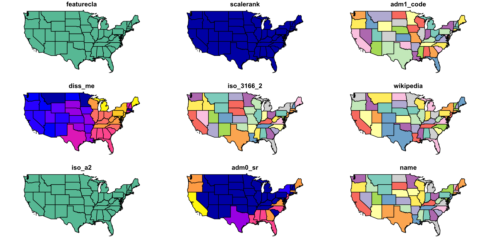
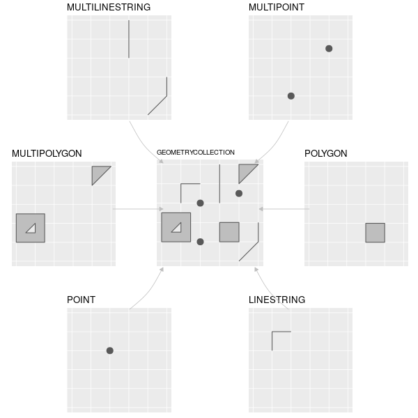
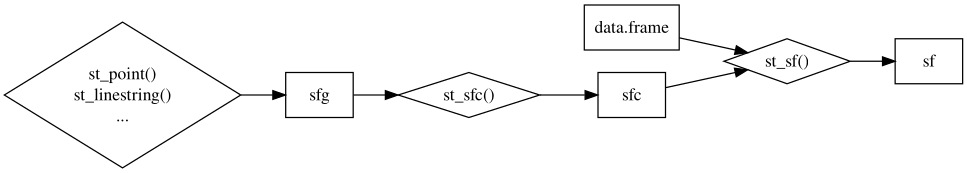
vectormodel relies onsimple features: points, lines, and polygons (coordinates) sfis the main R package for working with vector data- an
sfobject should have three things:- attributes (what: data frame)
- features (where: geometry column)
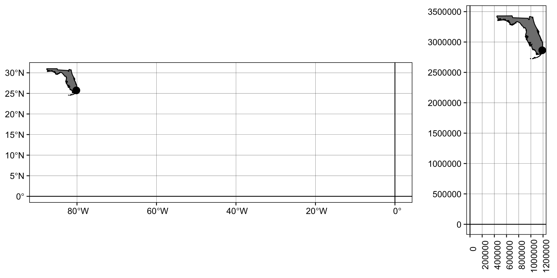
- CRS (in relation to what?: in the header)
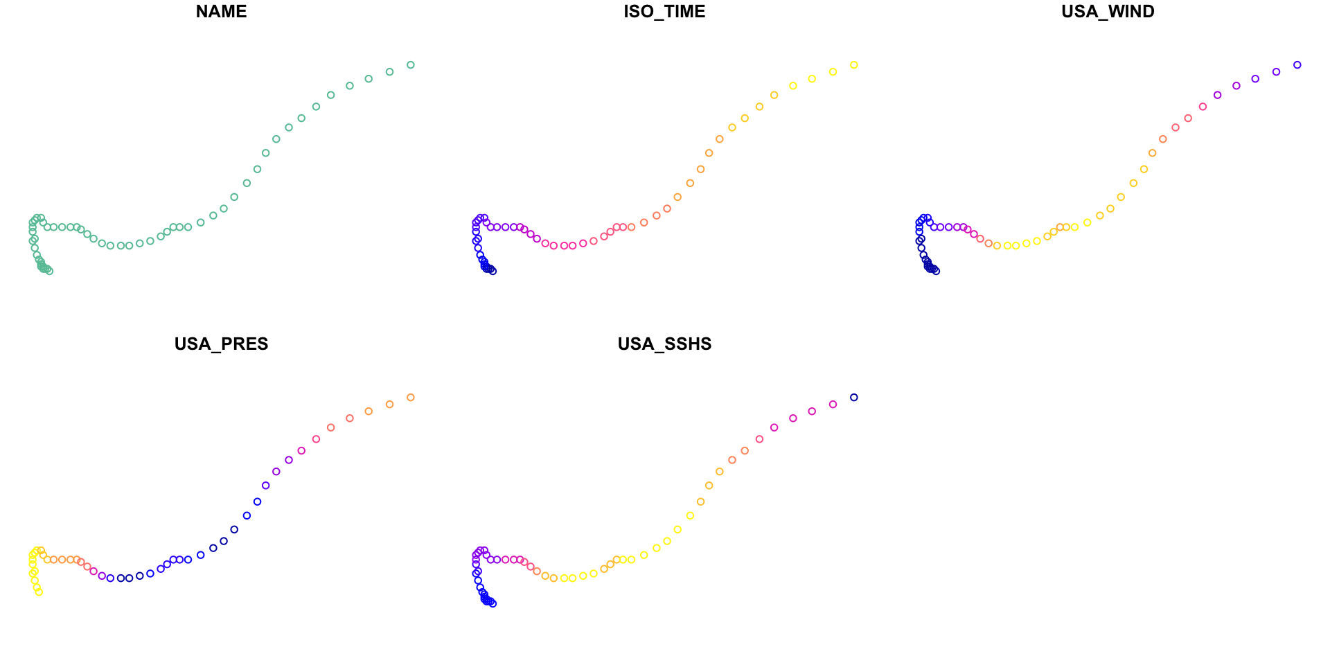
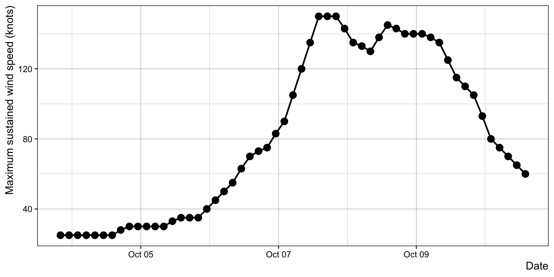
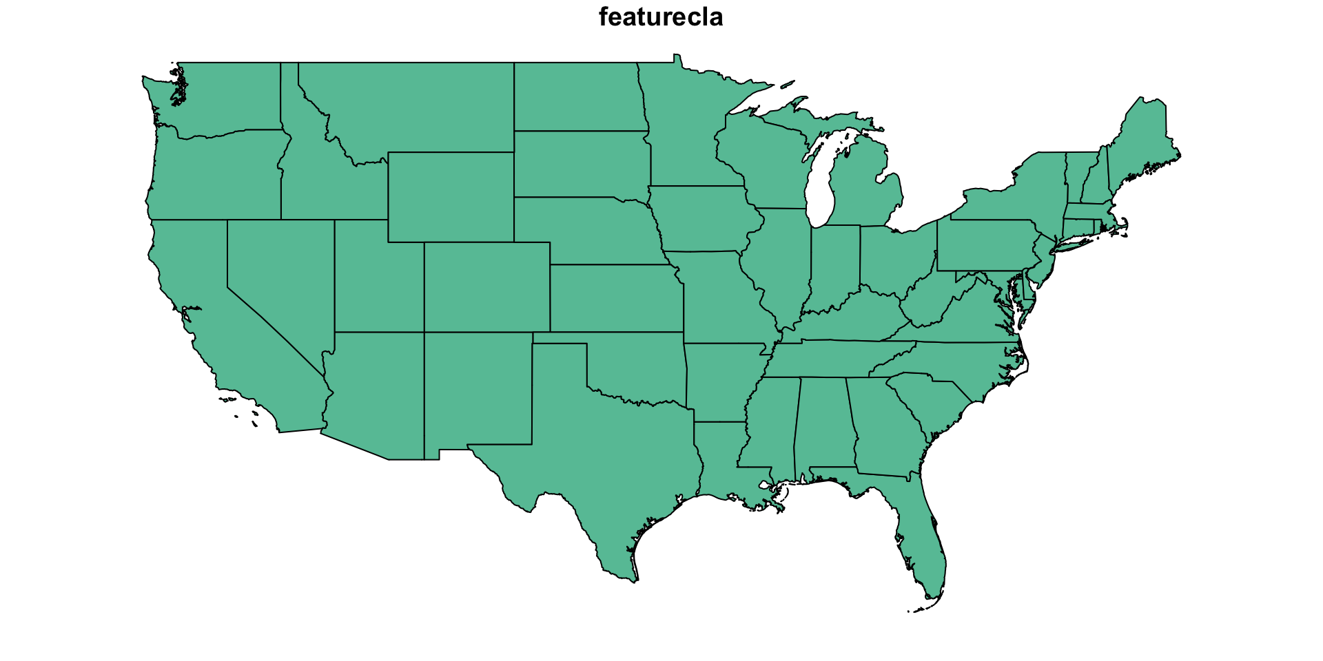
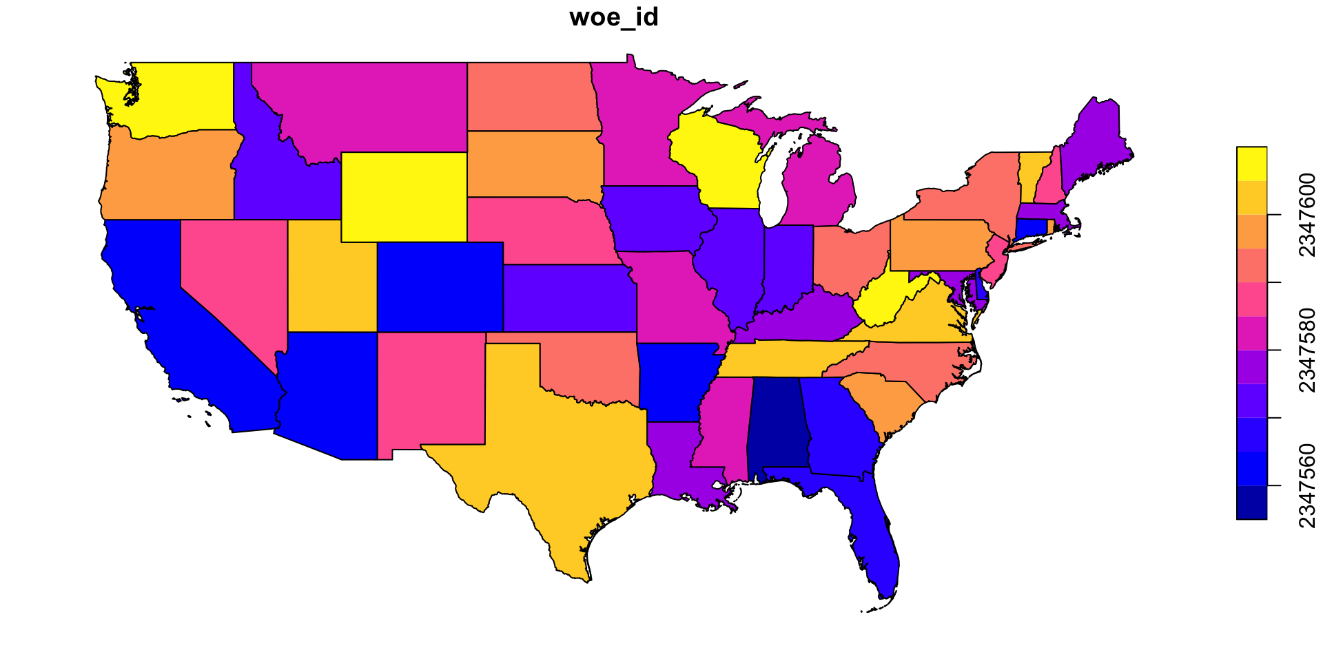
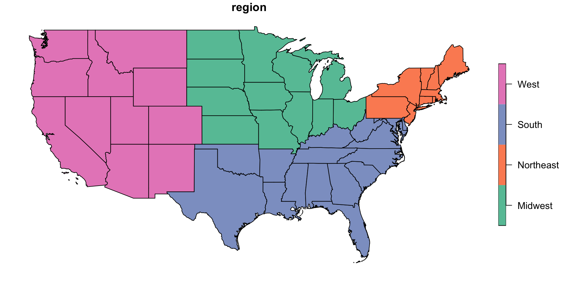
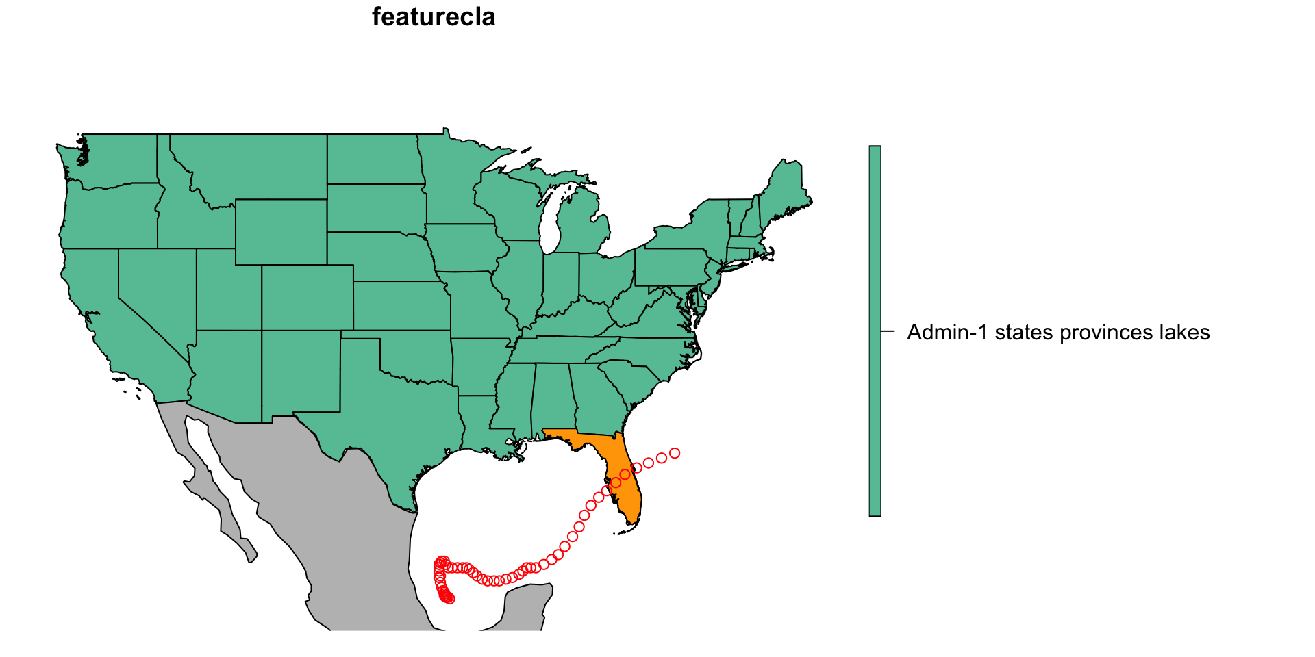
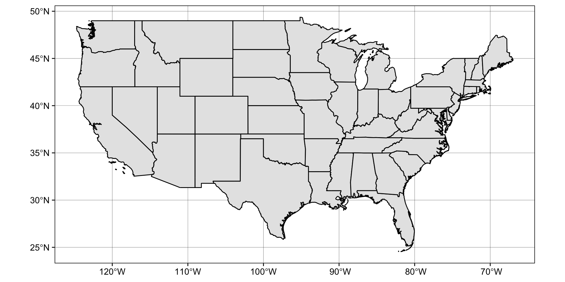
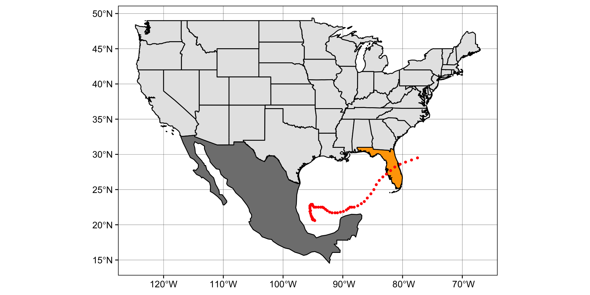
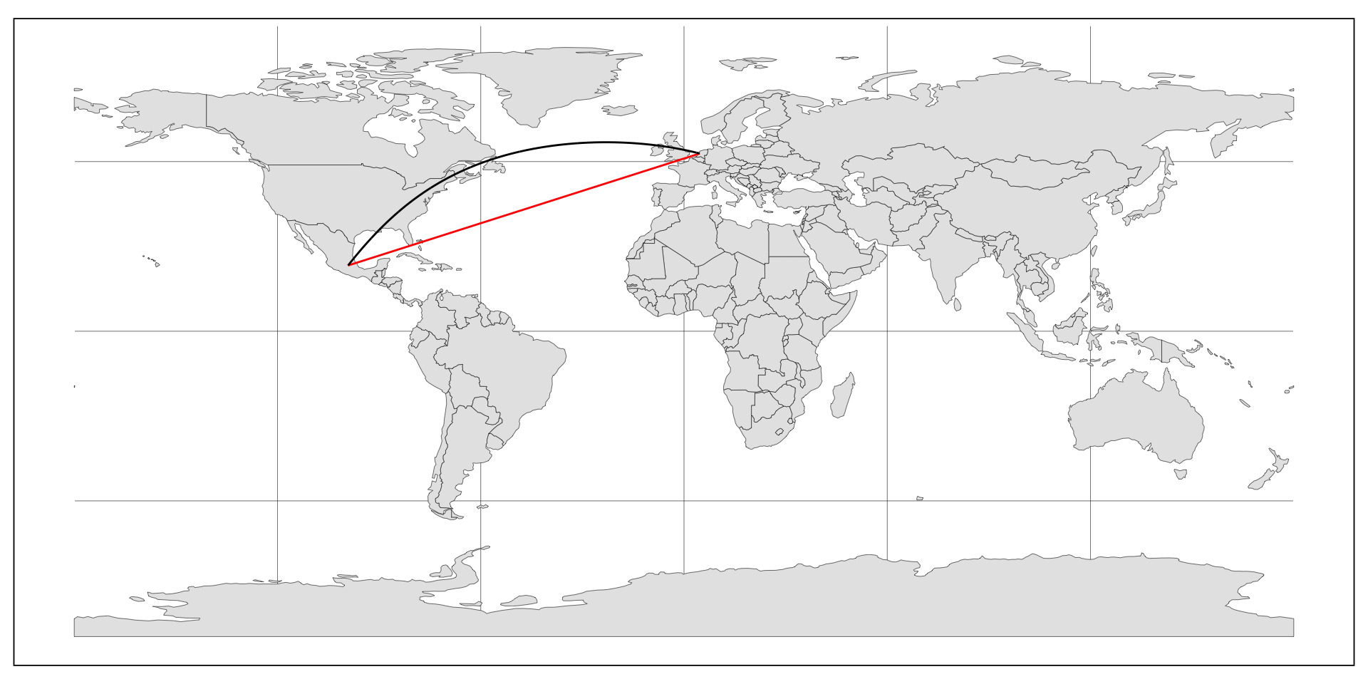
sfobjects can be treated liketibbles/data.frames- Quickly visualize sf objects using
plot(),ggplot(), ormapview()