EVR 628- Intro to Environmental Data Science

Working with spatial data in R

Juan Carlos Villaseñor-Derbez (JC)

Announcements

Upcoming EVR Seminar

Travis Coan, Professor of Computational Social Science, University of Exeter

Last Week

• Spatial data can be represented in a vector model, or a raster model
• We focused on vector data, which is represented by points, lines, polygons (and combination of these)
• vector data are often saved as shapefiles, geoJSON files, or geopackage files
• In R, we use the simple features standard to work with vector data via {sf}
• Regardless of the file extension (.shp, .gpkg…), we read them with sf::read_sf()
• sf objects have three main components:
  • CRS: Where is the origin
  • geometry: The spatial portion of the data
  • attributes: The characteristics associated to each point, line, or polygon

Learning Objectives

By the end of this week, you should be able to

• Identify whether a map was built with raster or vector data (or both)
• Load and work with raster objects with {terra}
• Visualize and manipulate raster data with {tidyterra}

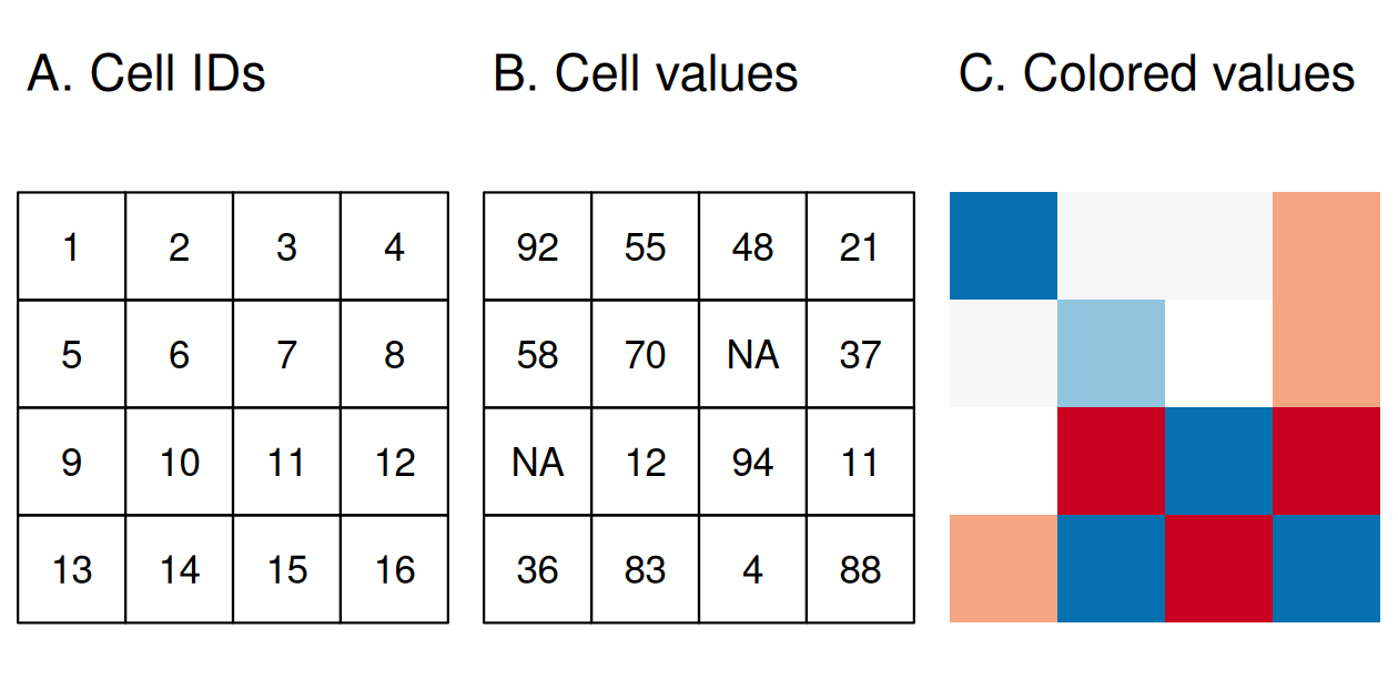
Raster Data Model

Raster Data Model

• The world is represented with a continuous grid
• Grid is made up of grid cells or pixels
• All pixels are the same size¹
• For most applications, grid cells will be “square”

1. The definition of “size” will depend on the coordinate reference system

Raster Data Model

• Polygon
• Raster (low res: 0.1°)
• Raster (high res: 0.01°)

plot(FL_counties_rast_high)

Raster Data Model

Common Applications:

• Usually used to represent continuous information:
  • Elevation / Depth
  • Temperature
  • Population density
  • Spectral data (in remote sensing applications)
• Discrete data can also be used

Raster Data Model

Common extensions include:

• .tiff / .tif:
  • “Tagged Image File Format”
• .asc
• .nc: Common in remote sensing and climate model output

TIFF or “GeoTiff” is simply an image made of pixels

Components of a Raster Object

• Two main components:
  • Header: metadata with CRS, extent, and origin
  • Matrix: the data we want to represent

• x-coordinates = columns
• y-coordinates = rows
• In terra the “origin” of the matrix is the top-left corner

Source: Wickham, Cetinkaya-Rundel, and Grolemund (2023)

Raster Is Faster. . . But Why?

• There is a fundamental relationship between resolution, extent, and origin:

\[ \mathrm{resolution_x} = \frac{x_{max} - x_{min}}{n_{col}} \]

• Raster data are typically “lighter” (and faster to work with) because we don’t need to store the coordinates for all corners of each cell

Q: How many coordinates does R need to store if you specify the origin, extent, and resolution?

A: One coordinate pair, lattitude and longitude for the origin

• In contrast to vector data, the cell of one raster layer can only hold a single value

Raster Is Faster. . . But Why?

Source: Wickham, Cetinkaya-Rundel, and Grolemund (2023)

• I just need to store the coordinates for the center of cell #1
• Coordinates for cell number 2 are \((X_1 + resolution, Y_1)\)

Raster Data in R

The terra Package

{terra}: An R package to work with raster datasets

The {terra} package:

• Replaces the older {raster} package
• Provides functions to create, read, transform, manipulate, and export raster data
• Has its own approach to vector data (not friendly with the tidyverse)
• Still plays well with sf

The terra Package: Example

• I can read a raster file into using the function rast()

library(terra) # Load terra
# Load in my raster
depth <- rast("data/raw/depth_raster.tif")
depth # Printing a raster reveals the header, not the data

class       : SpatRaster 
size        : 3600, 7200, 1  (nrow, ncol, nlyr)
resolution  : 0.05, 0.05  (x, y)
extent      : -180, 180, -90, 90  (xmin, xmax, ymin, ymax)
coord. ref. : lon/lat WGS 84 (EPSG:4326) 
source      : depth_raster.tif 
name        :       depth_m 
min value   : -10273.276367 
max value   :      0.985951 

• Q: What is the resolution of this raster?
• A: 0.05°
• Q: What is the extent?
• A: The world

Find info contained in the header with specific functions:

ext(depth)   # Gets the extent

SpatExtent : -180, 180, -90, 90 (xmin, xmax, ymin, ymax)

res(depth)   # Gets the resolution

[1] 0.05 0.05

dim(depth)   # Returns nrow, ncol, nlayers

[1] 3600 7200    1

ncell(depth) # Number of pixels (values)

[1] 25920000

names(depth) # Gets the names for each layer

[1] "depth_m"

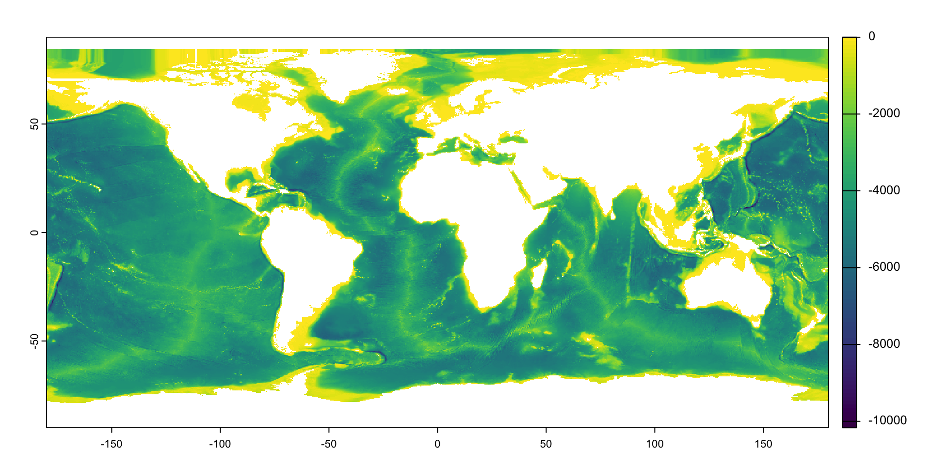
Visualizing Rasters in R

The fastest way is to use the base plot() function

plot(depth) # Single line of code gets me a decent map

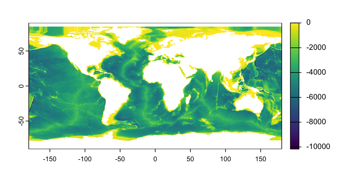
Visualizing Rasters in R

As with vector data, I can layer different pieces of my plot

plot(depth) # Build plot
plot(FL_counties, add = T) # Add FL counties on top

• Q: How are missing values represented?
• A: As transparent (white) pixels

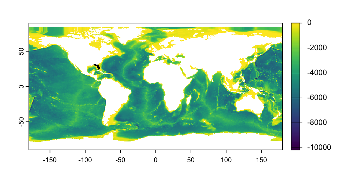
Manipulating Raster Objects

Task: Produce a map of water depth around FL

• Q: In human language, what do I have to do?
• A: “Zoom-in” on my global raster: crop()¹

FL_depth <- crop(depth, FL_counties) # Crop the global depth raster to the extent of FL_counties
plot(FL_depth)
plot(FL_counties, add = T)

1. Note that in terra::crop() does the same as sf::st_crop(), but for rasters

Manipulating Raster Objects

Task: Build the same map, but only show shallow (depth > -100 m) waters

• Rasters are just matrices, so we can use our trusty binary operators

plot(FL_depth <= -100)

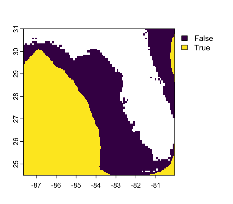
Manipulating Raster Objects

Task: Build the same map, but only show shallow (depth > -100 m) waters

• In a data.frame (or sf) object, you can remove rows (observations) based on values
• But a raster is not a tidy table. It’s a matrix, so removing rows wouldn’t be wise
• Instead of filtering data, we turn them into NA

# Crop FL
FL_depth <- crop(depth, FL_counties)
# Find pixels deeper than 100 and replace them with NA
FL_depth[FL_depth <= -100] <- NA
# Plot it
plot(FL_depth)
plot(FL_counties, add = T)

• This code is not very readable

Tidy rasters in R: {tidyterra}

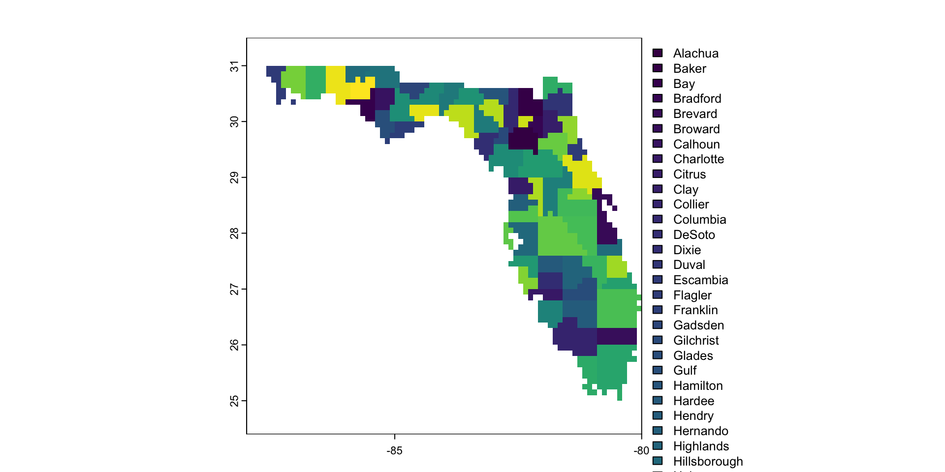
Tidy Rasters in R: {tidyterra}

{tidyterra}: Common methods of the tidyverse for objects created with {terra}

The {tidyterra} package:

• Developed by Diego Hernangómez (Hernangómez (2023))
• Extends, but doesn’t replace, the terra package
• Provides functions to manipulate and visualize the attribute portion of the raster
• Brings ggplot capabilities (geom_spatraster())

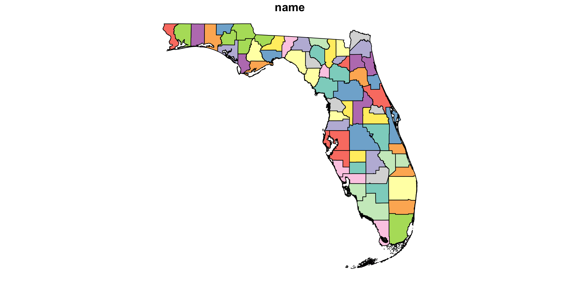
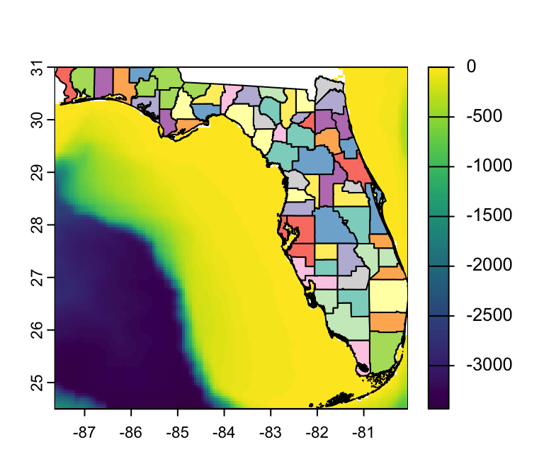
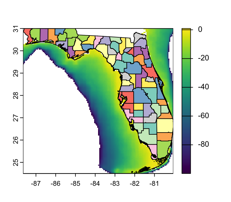
Visualizing Rasters in R: {tidyterra}

library(tidyterra) # Load terra
ggplot() +         # Begin a ggplot
  geom_spatraster(data = depth, # specify object to plot
                  aes(fill = depth_m)) + # specify layer to plot
  geom_sf(data = FL_counties) # Add FL counties on top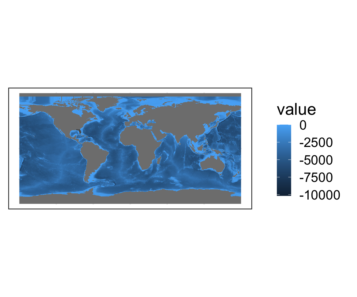

• Q: How are missing values represented?
• A: As gray pixels

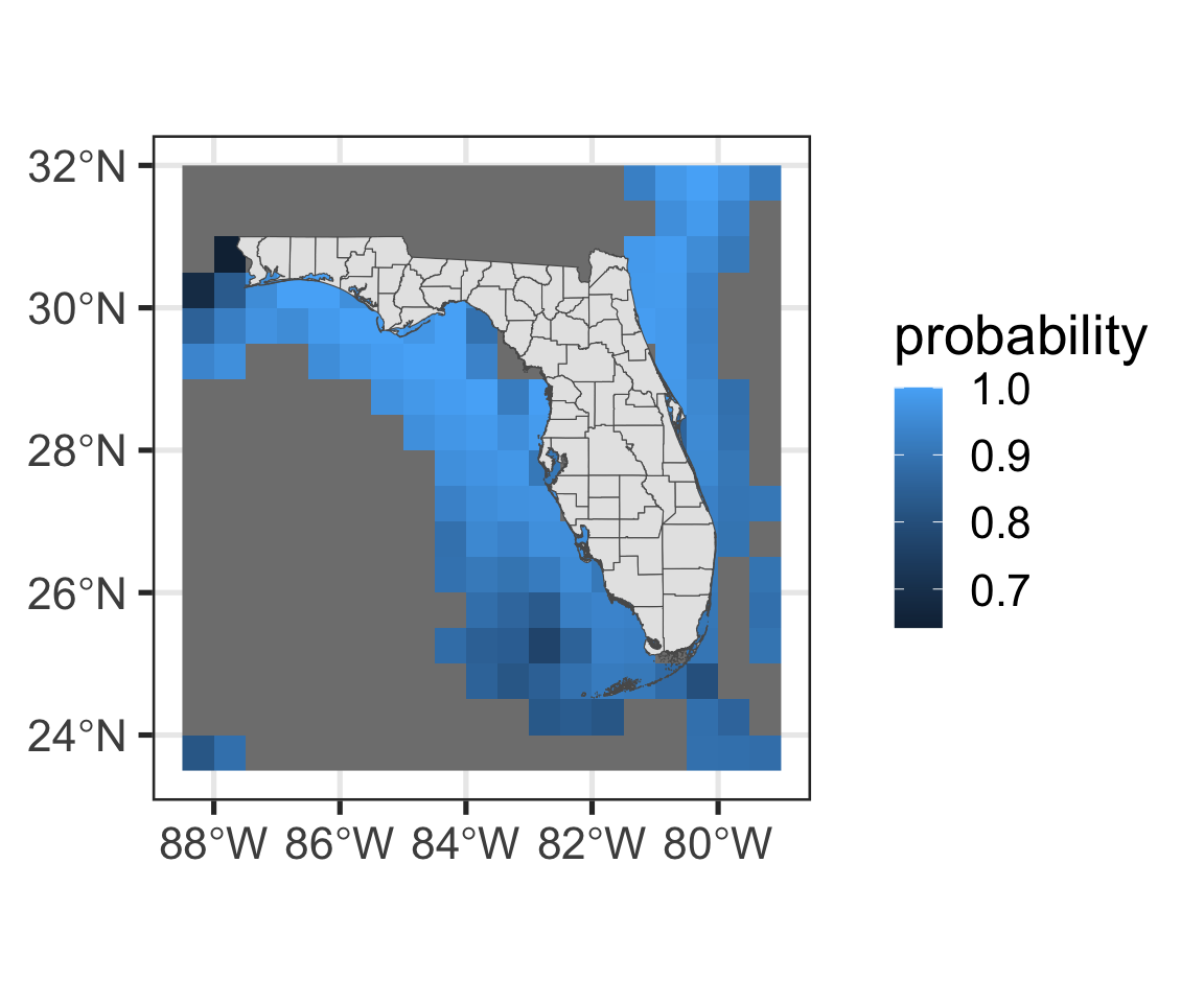
Manipulating Rasters with tidyterra

library(tidyterra)
FL_depth <- depth |> 
  terra::crop(FL_counties) |> 
  tidyterra::filter(depth_m >= -100)

plot(FL_depth)
plot(FL_counties, add = T)

Remember:

• terra for the spatial part (e.g. crop())
• tidyterra for the attribute part (e.g. filter())

Rasters with more than one attribute (layer)

Combining Rasters in terra

Source: Wasser et al., 2024

All layers must have the same extent and resolution

Combining Rasters in terra

# Let's read habitat suitability models for four sea turtle species
log <- rast("data/raw/AquaMaps/Caretta_caretta.tiff")
green <- rast("data/raw/AquaMaps/Chelonia_mydas.tiff")
leather <- rast("data/raw/AquaMaps/Dermochelys_coriacea.tiff")
hawk <- rast("data/raw/AquaMaps/Eretmochelys_imbricata.tiff")
# We can combine them together using the `c()` function
turtles <- c(log, green, leather, hawk)
turtles

class       : SpatRaster 
size        : 300, 720, 4  (nrow, ncol, nlyr)
resolution  : 0.5, 0.5  (x, y)
extent      : -180, 180, -75, 75  (xmin, xmax, ymin, ymax)
coord. ref. : lon/lat WGS 84 (EPSG:4326) 
sources     : Caretta_caretta.tiff  
              Chelonia_mydas.tiff  
              Dermochelys_coriacea.tiff  
              Eretmochelys_imbricata.tiff  
names       : Caretta_caretta, Chelonia_mydas, Dermoch~oriacea, Eretmoc~bricata 
min values  :            0.01,           0.01,            0.01,            0.01 
max values  :            1.00,           1.00,            1.00,            1.00 

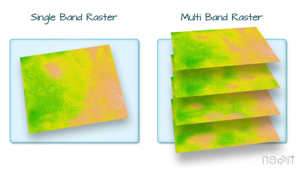
Multi-Layer Rasters

Calling plot() on a multi-layer raster shows us one sub-plot per layer

plot(turtles)

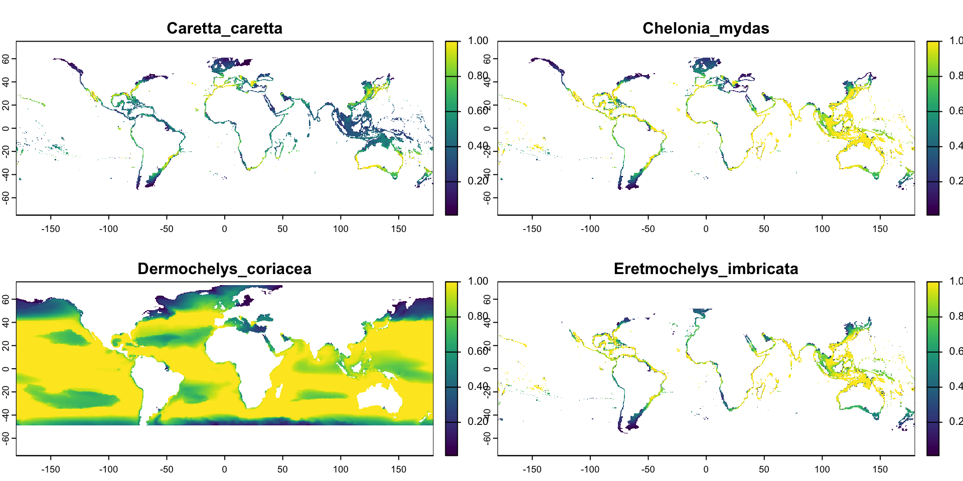
Multi-Layer Rasters

Task: Calculate the mean habitat suitability around FL waters

turtle_habitat <- turtles |> # Start from turtles
  # And pipe into filter()
  filter(Caretta_caretta > 0.5,
         Chelonia_mydas > 0.5,
         Dermochelys_coriacea > 0.5,
         Eretmochelys_imbricata > 0.5)
# Inspect the metadata
turtle_habitat
# And plot it
plot(turtle_habitat)

class       : SpatRaster 
size        : 300, 720, 4  (nrow, ncol, nlyr)
resolution  : 0.5, 0.5  (x, y)
extent      : -180, 180, -75, 75  (xmin, xmax, ymin, ymax)
coord. ref. : lon/lat WGS 84 (EPSG:4326) 
source(s)   : memory
names       : Caretta_caretta, Chelonia_mydas, Dermoch~oriacea, Eretmoc~bricata 
min values  :            0.51,           0.51,            0.55,            0.51 
max values  :            1.00,           1.00,            1.00,            1.00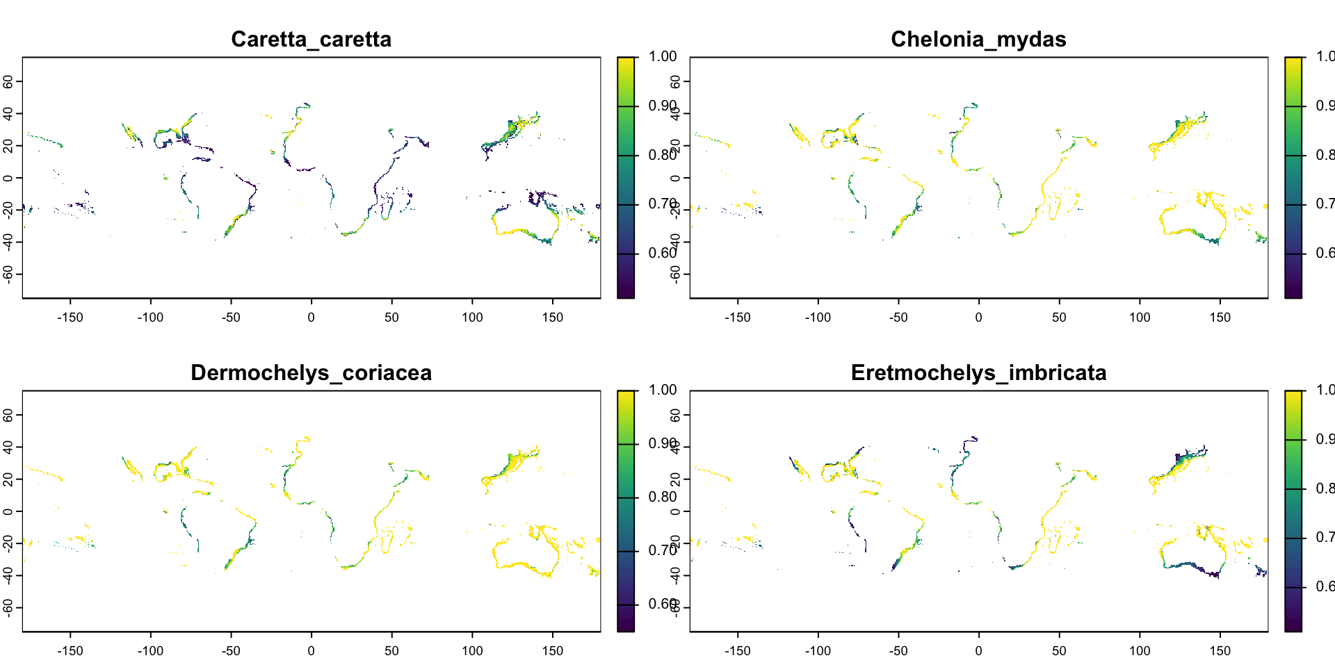 

Multi-Layer Rasters

Task: Calculate the mean habitat suitability around FL waters

turtle_habitat <- turtles |> # Start from turtles
  # And pipe into filter()
  filter(Caretta_caretta > 0.5,
         Chelonia_mydas > 0.5,
         Dermochelys_coriacea > 0.5,
         Eretmochelys_imbricata > 0.5) |> 
  # Then crop it to FL counties
  crop(st_buffer(FL_counties, dist = 100000)) |>  # Any guesses on what st_buffer is doing?
  mean()

Wrap Up

• Raster Data Model: Continuous grid representation with pixels/cells of uniform size
  • Ideal for continuous data (elevation, temperature, population density)
  • More storage-efficient than vector data
  • Each cell holds a single value per layer
• The terra Package:
  • Modern replacement for {raster} package
  • Use rast() to read raster files (.tif, .tiff, .asc, .nc)

• The tidyterra Package:
  • Extends terra with tidyverse-friendly functions
  • Use terra for spatial operations (e.g., crop())
  • Use tidyterra for attribute operations (e.g., filter(), mutate())
• Multi-Layer Rasters:
  • Combine multiple rasters with c()
  • All layers must have same extent and resolution
  • Use mean(), sum(), etc. to aggregate across layers

Before Next Class:

• Update RStudio
• Install terra, tidyterra, and ggspatial

install.packages("terra")
install.packages("tidyterra")
install.packages("ggspatial")

References

Hernangómez, Diego. 2023. “Using the Tidyverse with Terra Objects: The Tidyterra Package.” Journal of Open Source Software 8 (91): 5751. https://doi.org/10.21105/joss.05751.

Wickham, Hadley, Mine Cetinkaya-Rundel, and Garrett Grolemund. 2023. R for Data Science: Import, Tidy, Transform, Visualize, and Model Data. 2nd ed. Sebastopol, CA: O’Reilly Media.