Factors, Dates, and Strings of Text
EVR 628- Intro to Environmental Data Science
Rosenstiel School of Marine, Atmospheric, and Earth Science and Institute for Data Science and Computing
Today’s Agenda
What We’ll Cover
- Factors - Working with ordinal categorical data
- Dates & Times - Temporal data analysis
- Strings - Text manipulation and cleaning
- Regular Expressions - Pattern matching in text
Key Takeaways
- Factors: Use
forcatsfor categorical data manipulation - Dates: Use
lubridatefor temporal data analysis - Strings: Use
stringrfor text manipulation - Regex: Learn patterns for powerful text processing
My two cents
- It would take me months to cover all functions in these three packages
- You should be paying attention to the general approach
- Don’t attempt to build a list of if problem is X then I need to use Y function
Part 1: Factors
Working with Ordinal Categorical Data
What Are Factors?
- Categorical variables with fixed and known set of possible values
- Allow us to control the order in which character vectors appear (other than alphabetical)
- Useful for modelling because establish an identity or sequence between possible values
Why Do We Need Factors?
Imagine you record the month in which some observation took place
Using a character string to record this has two problems:
- It doesn’t sort in a useful or intuitive way
- We know there are only twelve possible months, but character strings are susceptible to typos that R will ignore
Why Do We Need Factors?
- Factors allow us to avoid these two downsides
# Specify the levels (all possible values, and their order)
month_levels <- c("Jan", "Feb", "Mar", "Apr", "May", "Jun",
                  "Jul", "Aug", "Sep", "Oct", "Nov", "Dec")
months_factor <- factor(x = months, levels = month_levels) # Build my factor
months_factor
[1] Dec Apr Jan Mar
Levels: Jan Feb Mar Apr May Jun Jul Aug Sep Oct Nov Dec[1] Jan Mar Apr Dec
Levels: Jan Feb Mar Apr May Jun Jul Aug Sep Oct Nov Dec- What about typos?
Creating Factors in the Tidyverse
- Instead of
factor()we useforcats::fct()
The {forcats} Package
![]()
{forcats}: A suite of tools that solve common problems with factors
Key forcats functions:
fct_reorder()- Reorder factor levels based on datafct_relevel()- Reorder factor levels by handfct_lump_*()- Group small categories- There are many others
Today’s data #1
#You will need to reinstall the package: remotes::install_github("jcvdav/EVR628tools")
library(EVR628tools)
# Load the geartypes data
data("data_geartypes")
data_geartypes
# A tibble: 840 × 3
vessel_id geartype effort_hours
<chr> <chr> <dbl>
1 00319684b-b03f-3b96-7560-0750e4b828fa TRAWLERS 2.22
2 00618559b-b68c-f85c-df65-112808b97e68 OTHER_PURSE_SEINES 577.
3 0091ceee9-9421-e3bc-9c5a-6d854975545c TUNA_PURSE_SEINES 17.0
4 00e3bfcdd-de86-c933-dbd1-a6c354a40f2c TRAWLERS 3226.
5 00e410e76-6d15-b0ad-4b4e-3b086cb9eb81 TRAWLERS 1484.
6 0108b3937-772f-d55b-aeb7-1c6113ac1722 TRAWLERS 474.
7 01391f16b-b01b-3527-c87e-c252b6054037 TRAWLERS 503.
8 0144ae898-893a-5fca-3029-d6f4d9e1c6cf TRAWLERS 286.
9 01654f527-7d77-76e3-e085-21c60790c557 TRAWLERS 233.
10 01dbe4ace-ee89-a70e-3136-11b42bbebeb7 POLE_AND_LINE 3.31
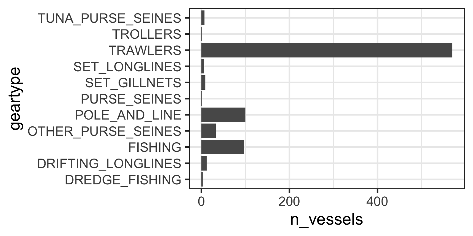
# ℹ 830 more rowsTask: Number of vessels by geartype?
- Check the documentation
- Use my data tidying skills
# Example: Total activity by gear type
gear_summary <- data_geartypes |>
  group_by(geartype) |>
  summarize(n_vessels = n_distinct(vessel_id)) |>
  arrange(desc(n_vessels))

gear_summary
# A tibble: 11 × 2
geartype n_vessels
<chr> <int>
1 TRAWLERS 570
2 POLE_AND_LINE 100
3 FISHING 97
4 OTHER_PURSE_SEINES 33
5 DRIFTING_LONGLINES 12
6 SET_GILLNETS 9
7 TUNA_PURSE_SEINES 7
8 SET_LONGLINES 6
9 DREDGE_FISHING 3
10 PURSE_SEINES 2
11 TROLLERS 1Reordering Factor Levels
When our data are already assembled, we can modify the order in which factor levels appear
This doesn’t modify the values, just the order in which they are interpreted
Reordering Factor Levels
Use
fct_reorder()Look at the documentation for two crucial arguments:
.fWhat is your soon-to-be factor?.xWhat is the variable by which you want to order your factor?
gear_summary <- data_geartypes |>
  group_by(geartype) |>
  summarize(n_vessels = n_distinct(vessel_id)) |>
  arrange(desc(n_vessels)) |>
  mutate(geartype = fct_reorder(.f = geartype, .x = n_vessels))
gear_summary
# A tibble: 11 × 2
geartype n_vessels
<fct> <int>
1 TRAWLERS 570
2 POLE_AND_LINE 100
3 FISHING 97
4 OTHER_PURSE_SEINES 33
5 DRIFTING_LONGLINES 12
6 SET_GILLNETS 9
7 TUNA_PURSE_SEINES 7
8 SET_LONGLINES 6
9 DREDGE_FISHING 3
10 PURSE_SEINES 2
11 TROLLERS 1Reordering Factor Levels
My ggplot code now produces the expected figure
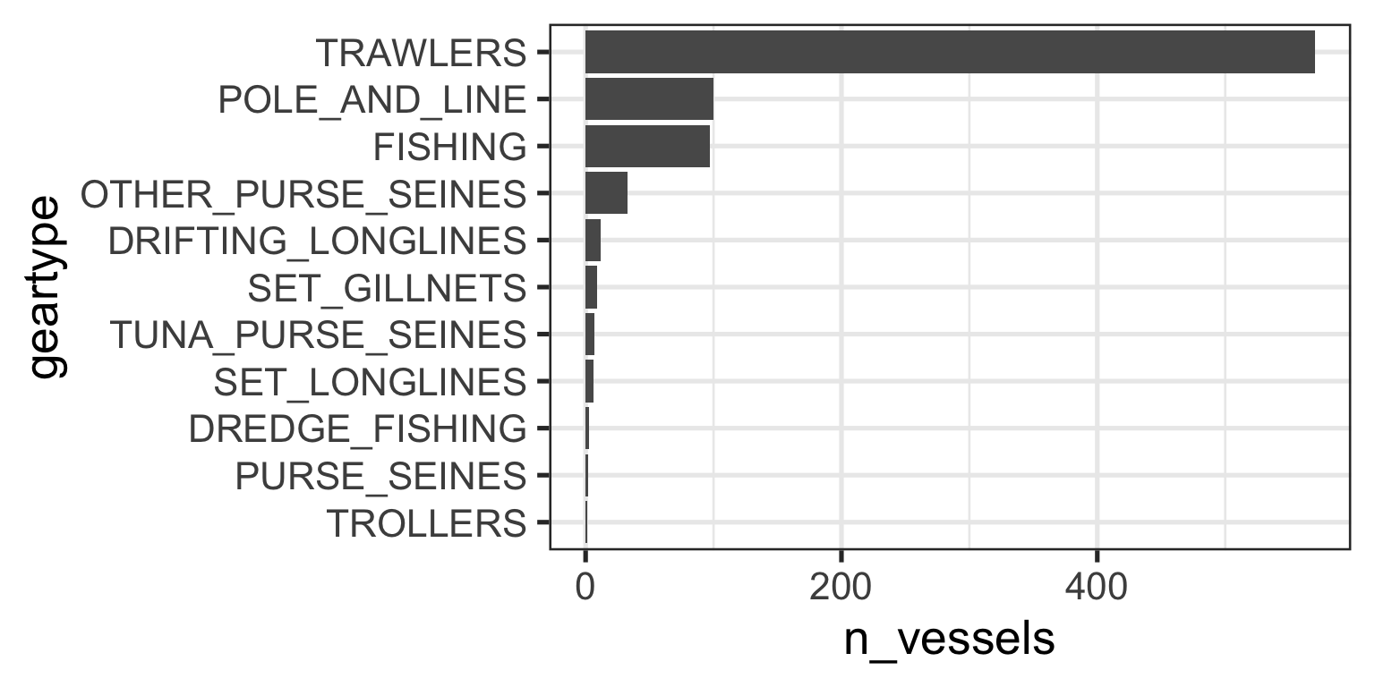
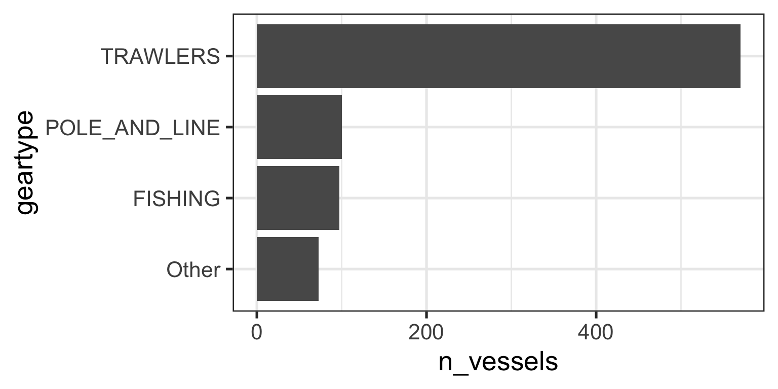
Lumping Small Categories
- It is clear that three gears dominate the data
- Let’s
lumpall other gears into a new category of “others” - I will use the
fct_lump_n()function.It does modify values - Check documentation here for other versions
gear_summary <- data_geartypes |>
  mutate(geartype = fct_lump_n(f = geartype, n = 3)) |>     # Keep top 3, lump the rest)
  group_by(geartype) |>
  summarize(n_vessels = n_distinct(vessel_id)) |>
  arrange(desc(n_vessels)) |>
  mutate(geartype = fct_reorder(.f = geartype, .x = n_vessels)) # Then reorder based on new n by groups
gear_summary
# A tibble: 4 × 2
geartype n_vessels
<fct> <int>
1 TRAWLERS 570
2 POLE_AND_LINE 100
3 FISHING 97
4 Other 73Lumping Small Categories
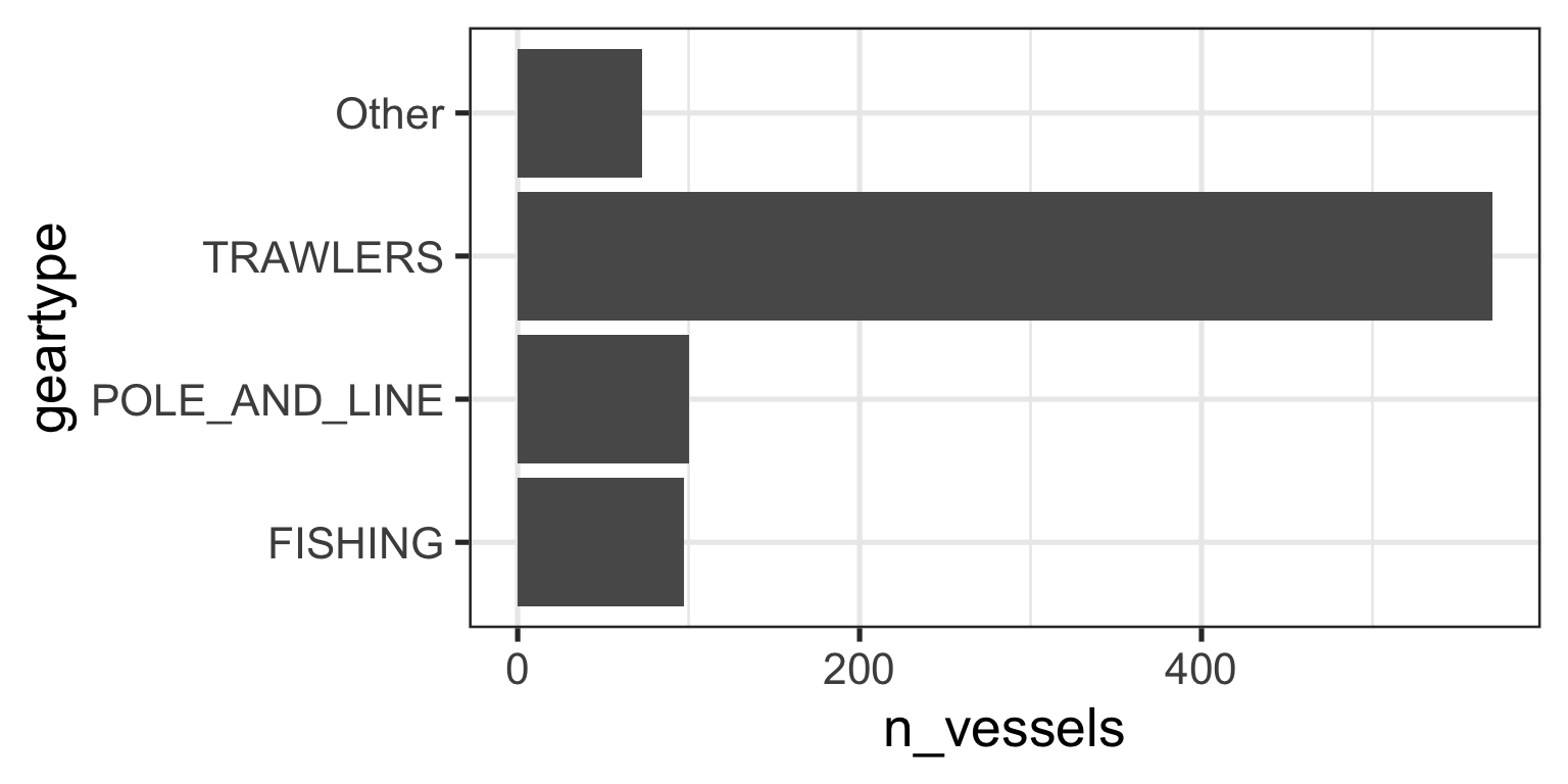
Reordering Factor Levels by hand
- You can manually change the order of factor levels with
fct_relevel
gear_summary <- data_geartypes |>
  mutate(geartype = fct_lump_n(f = geartype, n = 3)) |>     # Keep top 3, lump the rest)
  group_by(geartype) |>
  summarize(n_vessels = n_distinct(vessel_id)) |>
  arrange(desc(n_vessels)) |>
  mutate(geartype = fct_reorder(.f = geartype, .x = n_vessels), # Then reorder based on new n by groups
         geartype = fct_relevel(.f = geartype, c("FISHING", "POLE_AND_LINE", "TRAWLERS", "Other")))
gear_summary
# A tibble: 4 × 2
geartype n_vessels
<fct> <int>
1 TRAWLERS 570
2 POLE_AND_LINE 100
3 FISHING 97
4 Other 73Did anything change?
Reordering Factor Levels by hand
Recoding Factor Levels
- What if we want to create multiple groups, rather than just “Others”?
- We can use
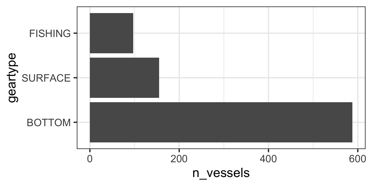
fct_collapseto manually specify which values should be collapsed into new levels. - For example, we might want to collapse our raw gear types into bottom gear and surface gear
gear_summary <- data_geartypes |>
  mutate(geartype = fct_collapse(geartype,
                                 "BOTTOM" = c("DREDGE_FISHING", "SET_GILLNETS",
                                              "SET_LONGLINES", "TRAWLERS"),
                                 "SURFACE" = c("DRIFTING_LONGLINES", "OTHER_PURSE_SEINES",
                                               "POLE_AND_LINE", "PURSE_SEINES",
                                               "TROLLERS", "TUNA_PURSE_SEINES"))) |>
  group_by(geartype) |>
  summarize(n_vessels = n_distinct(vessel_id))

gear_summary # Unspecified factor levels are left unmodified
# A tibble: 3 × 2
geartype n_vessels
<fct> <int>
1 BOTTOM 588
2 SURFACE 155
3 FISHING 97Recoding Factor Levels
Other fct_* functions
- There are 30+ functions to help you
- Look at the package documentation here
Part 2: Dates and Times
Working with Temporal Data
Parts of a Date/Time Object
In R, there are three types of date/time data that point at an instant in time:
- A date - In a tibble, you will see it as
<date> - A time - A tibble will print it as
<time> - A date-time - The combination of a date and a time. Tibbles will print it as
<dttm> - Strive to work with the simplest version of the data type
Note
- Here and there you might hear about
POSIXctandPOSIXltPOSIXstands for “Portable Operating System Interface”, a Unix standard- The
ctstands for “calendar time” (seconds elapsed since Jan 1, 1970) ltstands for “local time” (stores the human readable components)
Why Dates Are Tricky
Problems:
- Multiple formats
- Time zones
- Leap years, daylight saving time
The lubridate Package
![]()
{lubridate}: An R package that makes it easier to work with dates and times
Key lubridate functions:
- Create dates and times
- Get components form dates and times
- Deal with time spans
Creating Dates and Times
There are four approaches:
- When importing your data (if you are lucky)
- From character strings
- From individual components
- From other time-like classes (simply use
as_date()oras_datetime())
Creating Dates and Times when Importing Data
- Does your CSV file contain an ISO8601 date or date-time>
- Lucky you… you don’t need to do anything;
readrwill automatically recognize it - Note that US approach to dates is not standard, ISO8601 mandates that:
- Components are organized from biggest to smallest
- Date components are separated by
- - Time components are separated by
:(24 hr format, no am / pm) - Date is separated from time using
orT
Creating Dates and Times when Importing Data
If your csv file looks like this:
Then you can simply read it in:
# A tibble: 2 × 4
  class_date time_of_day combined             event
  <date>     <time>      <chr>                <chr>
1 2025-10-21 09:00       2025-10-21  09:00:00 class_starts
2 2025-10-21 10:15 2025-10-21 10:15:00 class_ends - If your date/time columns are not adhering to ISO standards
- You will need to use the
col_typesarguments inread_, as well ascol_date()orcol_datetime() - And specify the format in which the data were entered
Creating Date-Time Objects from Strings
- Lubridate provides multiple helpers
- If you know the order of your date/time components, you can infer which helper to use
- For example:
- What is the class of this object?
- What is the order of my components here?
- Likely
m,d,y, so I can use themdy()function
Creating Date-Time Objects from Strings
Let’s say your data looks like this:
So when you read them in, they look like this:
# A tibble: 10 × 2
   date        whales_observed
   <chr>                 <dbl>
 1 Jan-15-2024              12
 2 Jan-22-2024               8
 3 Feb-5-2024                7
 4 Feb-18-2024               8
 5 Mar-3-2024                7
 6 Mar-20-2024              12
 7 Apr-2-2024               14
 8 Apr-25-2024               8
 9 May-8-2024                6
10 May-30-2024               6
Notice that date is of class <chr>
Creating Date-Time Objects from Strings
Can I directly build a figure with date on the x-axis and # whales on the y-axis?
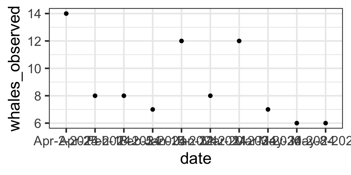
Nope…
Creating Date-Time Objects from Strings
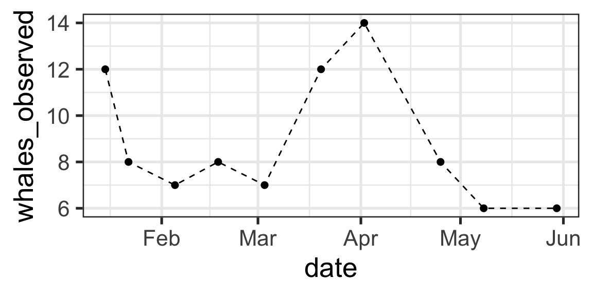
Steps:
- Identify the format of the date
- Use the appropriate
lubridatefunction to convert the string to a date - Plot my data
Creating Date-Time Objects from Strings
Steps:
- Identify the format of the date
- Use the appropriate
lubridatefunction to convert the string to a date - Plot my data
Creating Date-Time Objects from Strings
Steps:
- Identify the format of the date
- Use the appropriate
lubridatefunction to convert the string to a date - Plot my data
Creating Date-Time Objects from Strings
Steps:
- Identify the format of the date
- Use the appropriate
lubridatefunction to convert the string to a date - Plot my data
Creating Date-Time Objects from Strings
Many other helper functions
[1] "2025-10-21"[1] "2025-10-21"[1] "2025-10-21"[1] "2025-10-21 10:00:00 UTC"[1] "2025-10-21 12:00:00 UTC"- You just have to get your data into an acceptable format
- This will require you use your data tidying skills
Creating Date-Time Objects from Components
Sometimes you will not have a date column, and your data might look like this:
Creating Date-Time Objects from Components
- Then you can use the
make_date()ormake_datetime()functions - Note that these require
numericvalues (i.e. “Oct” won’t work, but10will)
whale_counts_dates <- whale_counts |>
  mutate(date = make_date(year, month, day)) |>
  select(date, whales_observed)

whale_counts_dates
# A tibble: 10 × 2
date whales_observed
<date> <dbl>
1 2025-01-15 12
2 2025-01-22 8
3 2025-02-05 7
4 2025-02-18 8
5 2025-03-03 7
6 2025-03-20 12
7 2025-04-02 14
8 2025-04-25 8
9 2025-05-08 6
10 2025-05-30 6Getting Components
- Sometimes we want to make calculations based on part of a date
- For example, how many whales did I observe per month?
# A tibble: 2 × 2
  date       whales_observed
  <date>               <dbl>
1 2025-01-15              12
2 2025-01-22 8- I can use
month()to extract the month of a date
Getting Components
Other useful functions
Time Spans
- Durations represent exact number of seconds
- Periods represent human units, like weeks and months
- Intervals represent a starting and end point
If you only care about physical time, use a duration; if you need to add human times, use a period; if you need to figure out how long a span is in human units, use an interval.
Subtracting two dates will give you a difftime object:
Duration vs Periods
[1] "2025-11-01 02:01:01 EDT"- Let’s add one day to this date
- What happened here? Daylight Saving Time ends on Nov 2, 2025 at 01:00
- These functions return different objects
Lubridate Is a Game Changer
- There are many functions that will help you with managing dates
- Whenever you have to work with dates, look at the package documentation
Part 3: Strings and Regular Expressions
Working with Characters
The stringr Package
![]()
{stringr}: a cohesive set of functions designed to make working with strings as easy as possible
Key functions allow you to:
- Extract data contained in strings
- Modify strings
- Create strings from data
Extract Data Contained in Strings
- A whale-watching company shared with you data on their trips
- The data look like this:
# A tibble: 4 × 3
  trip_id passengers notes
    <dbl>      <dbl> <chr>
1       1         25 Dolphins; whales
2       2         32 Whale; Sea lions
3       3         30 Sea lions; sea turtles
4 4 30 Sea lion; sea turtles - Your project requires presence / absence data, so the lack of abundances is not a problem
- Your whale-watching partners ask: How many people have seen each type of animal?
Extract Data Contained in Strings
tidyr offers four useful functions:
separate_longer_delim()andseparate_wider_delim()separate_longer_position()andseparate_wider_position()
separate_longer_delim() allows me to separate a column and make the data longer based on a delimiter:
Anything weird?
Modify Strings
The stringr package provides functions to modify, detect, and extract parts of strings
Let’s convert all letters to lowercase
sightings_tidy <- sightings |>
  separate_longer_delim(cols = notes, delim = "; ") |>
  rename(species = notes) |>
  mutate(species = str_to_lower(string = species))
sightings_tidy
# A tibble: 8 × 3
trip_id passengers species
<dbl> <dbl> <chr>
1 1 25 dolphins
2 1 25 whales
3 2 32 whale
4 2 32 sea lions
5 3 30 sea lions
6 3 30 sea turtles
7 4 30 sea lion
8 4 30 sea turtlesThere is also str_to_upper(), str_to_title(), and str_to_sentence()
Anything weird with these data?
Regular Expressions
Can I just remove the “s” to make everything singular?
The str_remove() function might help
sightings_tidy <- sightings |>
  separate_longer_delim(cols = notes, delim = "; ") |>
  rename(species = notes) |>
  mutate(species = str_to_lower(string = species),
         species = str_remove(string = species, pattern = "s"))
sightings_tidy
# A tibble: 8 × 3
trip_id passengers species
<dbl> <dbl> <chr>
1 1 25 dolphin
2 1 25 whale
3 2 32 whale
4 2 32 ea lions
5 3 30 ea lions
6 3 30 ea turtles
7 4 30 ea lion
8 4 30 ea turtlesOh no!
Regular Expressions
str_remove()will remove the first instance of the matched pattern- I need to remove the “
s” at the end of a word to make everything singular - To specify this complex pattern I need to use
regularexpressions ?regex
sightings_tidy <- sightings |>
  separate_longer_delim(cols = notes, delim = "; ") |>
  rename(species = notes) |>
  mutate(species = str_to_lower(string = species),
         species = str_remove(string = species, pattern = "s$")) # Match the "s" at the end of a line only
sightings_tidy
# A tibble: 8 × 3
trip_id passengers species
<dbl> <dbl> <chr>
1 1 25 dolphin
2 1 25 whale
3 2 32 whale
4 2 32 sea lion
5 3 30 sea lion
6 3 30 sea turtle
7 4 30 sea lion
8 4 30 sea turtleWe Can Now Answer the Question
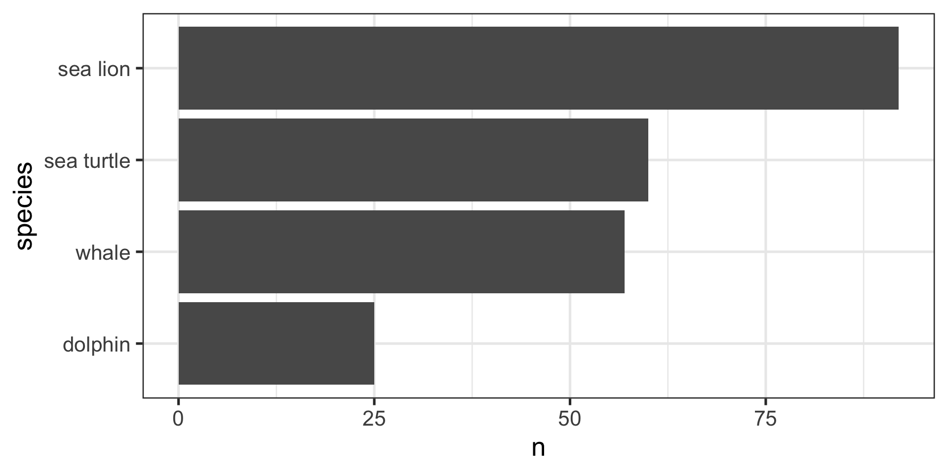
stringr is incredibly useful
Some functions:
- In combination with mutate:
str_replace()str_extract()str_split()str_sub()
- With
filter():str_detect()str_length()
- With
summarie():str_flatten()
Key Takeaways
- Factors: Use
forcatsfor categorical data manipulation - Dates: Use
lubridatefor temporal data analysis - Strings: Use
stringrfor text manipulation - Regex: Learn patterns for powerful text processing
Next Steps
- Practice with real datasets
- Combine these tools in data cleaning pipelines
- Explore advanced features as needed