EVR 628- Intro to Environmental Data Science

Data Tidying and Merging

Juan Carlos Villaseñor-Derbez (JC)

Learning Objectives

By the end of this week, you should be able to:

Understand the principles of tidy data
Transform data between wide and long formats using pivot_longer() and pivot_wider()
Merge datasets using different types of joins
Apply data tidying techniques to real-world messy datasets

Tidy Data

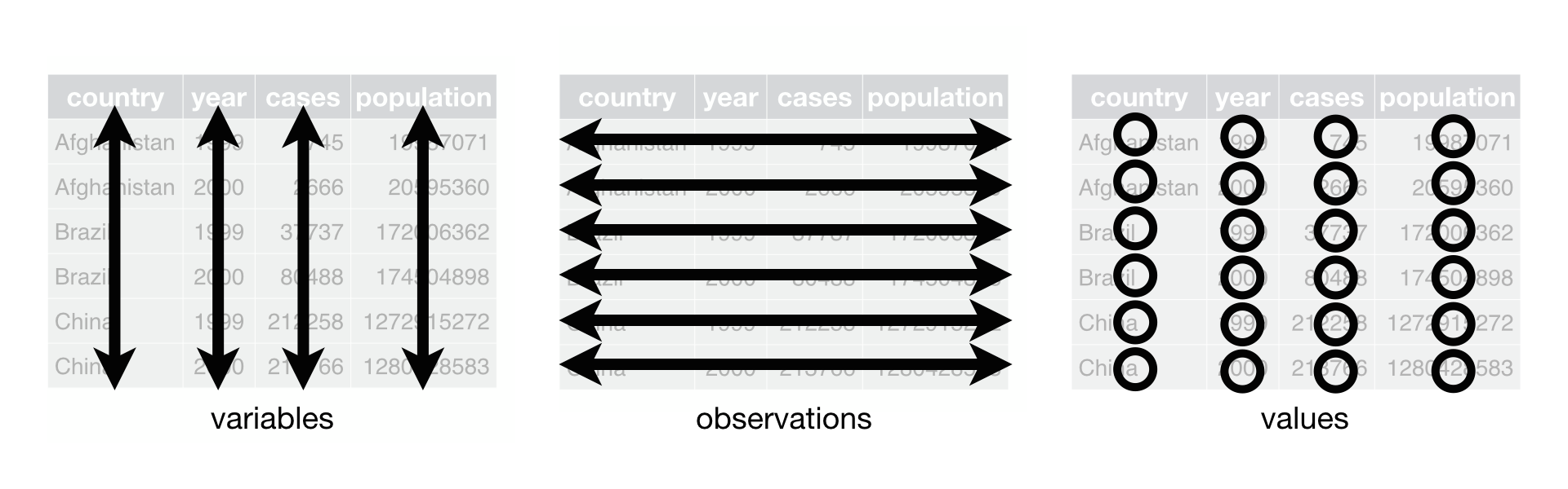
Image Credit: Wickham, Mine Cetinkaya-Rundel, and Grolemund (2023)

See Wickham (2014) for a full description of tidy data principles an the reshape2 package (old)

Messy Data?

“Tidy datasets are all alike, but every messy dataset is messy in its own way.”
— Hadley Wickham

Two main reasons for lack of tidy data:

Format was designed for data entry or human readability, not data analysis
No foresight

The `{tidyr}` Package

{tidyr}: A package for tidying data in R

Core functions:

Change the shape of your data with pivot_longer() and pivot_wider
Dealing with missing values with complete(), drop_na(), replace_na(), and fill() (not today)

Changing shape of data

Lengthening and widening with pivot_longer() and pivot_wider()

1) Lengthening data

Type of problem: Column names are values, not variables

Code

library(EVR628tools)
data("data_kelp")
data_kelp

# A tibble: 807 × 25
   location site  transect genus_species      TL_5 TL_10 TL_15 TL_20 TL_25 TL_30
   <chr>    <chr>    <dbl> <chr>             <dbl> <dbl> <dbl> <dbl> <dbl> <dbl>
 1 ASA      North        1 Alloclinus holde…    NA     1    NA    NA    NA    NA
 2 ASA      North        1 Caulolatilus pri…    NA    NA    NA     3    NA    NA
 3 ASA      North        1 Chromis punctipi…    NA    14    NA    NA    NA    NA
 4 ASA      North        1 Embiotoca jackso…    NA    NA    NA     6    NA    NA
 5 ASA      North        1 Embiotoca latera…    NA    NA    NA     1    NA    NA
 6 ASA      North        1 Girella nigricans    NA    NA    NA    NA     1    NA
 7 ASA      North        1 Hypsypops rubicu…    NA    NA    NA     4    NA    NA
 8 ASA      North        1 Oxyjulis califor…     2    61    46    NA    NA    NA
 9 ASA      North        1 Paralabrax clath…    NA    NA     1    NA    NA    NA
10 ASA      North        1 Sebastes carnatus    NA    NA    NA    NA     1    NA
# ℹ 797 more rows
# ℹ 15 more variables: TL_35 <dbl>, TL_40 <dbl>, TL_45 <dbl>, TL_50 <dbl>,
#   TL_55 <dbl>, TL_60 <dbl>, TL_65 <dbl>, TL_70 <lgl>, TL_75 <dbl>,
#   TL_80 <dbl>, TL_85 <dbl>, TL_90 <dbl>, TL_95 <dbl>, TL_100 <dbl>,
#   TL_105 <dbl>

Specifically: Total lengths are in column names instead of a total_length variable. There is no column for abundance.

Target

How should these data look like?

How many columns do we want?

What columns names do we want?

We want the data to be “longer”, with 6 columns:

location
site
transect
genus_species
total_length
abundance

The Messy Data Again

# A tibble: 5 × 25
  location site  transect genus_species       TL_5 TL_10 TL_15 TL_20 TL_25 TL_30
  <chr>    <chr>    <dbl> <chr>              <dbl> <dbl> <dbl> <dbl> <dbl> <dbl>
1 ASA      North        1 Alloclinus holderi    NA     1    NA    NA    NA    NA
2 ASA      North        1 Caulolatilus prin…    NA    NA    NA     3    NA    NA
3 ASA      North        1 Chromis punctipin…    NA    14    NA    NA    NA    NA
4 ASA      North        1 Embiotoca jacksoni    NA    NA    NA     6    NA    NA
5 ASA      North        1 Embiotoca lateral…    NA    NA    NA     1    NA    NA
# ℹ 15 more variables: TL_35 <dbl>, TL_40 <dbl>, TL_45 <dbl>, TL_50 <dbl>,
#   TL_55 <dbl>, TL_60 <dbl>, TL_65 <dbl>, TL_70 <lgl>, TL_75 <dbl>,
#   TL_80 <dbl>, TL_85 <dbl>, TL_90 <dbl>, TL_95 <dbl>, TL_100 <dbl>,
#   TL_105 <dbl>

We want to:

Identify columns starting with TL_
Send column names to a new column called total_length
Send the abundance values to to a new column called abundance

What do you expect the new dimensions of the data to be?

Solution: `pivot_longer()`

# Make it tidy
data_kelp |> # data_kelp goes into...
  pivot_longer(
    cols = starts_with("TL_"), #specify columns to pivot
    names_to = "total_length", # Where should column names be placed?
    values_to = "abundance")   # Where should values be placed?

# A tibble: 16,947 × 6
   location site  transect genus_species      total_length abundance
   <chr>    <chr>    <dbl> <chr>              <chr>            <dbl>
 1 ASA      North        1 Alloclinus holderi TL_5                NA
 2 ASA      North        1 Alloclinus holderi TL_10                1
 3 ASA      North        1 Alloclinus holderi TL_15               NA
 4 ASA      North        1 Alloclinus holderi TL_20               NA
 5 ASA      North        1 Alloclinus holderi TL_25               NA
 6 ASA      North        1 Alloclinus holderi TL_30               NA
 7 ASA      North        1 Alloclinus holderi TL_35               NA
 8 ASA      North        1 Alloclinus holderi TL_40               NA
 9 ASA      North        1 Alloclinus holderi TL_45               NA
10 ASA      North        1 Alloclinus holderi TL_50               NA
# ℹ 16,937 more rows

Are all my data there?

What’s up with all those NAs?

What type of data is in total_length and abundance?

Dealing with NAs

# Make it tidy
data_kelp |> # data_kelp goes into...
  pivot_longer(
    cols = starts_with("TL_"), #specify columns to pivot
    names_to = "total_length", # Where should column names be placed?
    values_to = "abundance",   # Where should values be placed?
    values_drop_na = TRUE)     # Specify that NA values should be removed)

# A tibble: 1,116 × 6
   location site  transect genus_species         total_length abundance
   <chr>    <chr>    <dbl> <chr>                 <chr>            <dbl>
 1 ASA      North        1 Alloclinus holderi    TL_10                1
 2 ASA      North        1 Caulolatilus princeps TL_20                3
 3 ASA      North        1 Chromis punctipinnis  TL_10               14
 4 ASA      North        1 Embiotoca jacksoni    TL_20                6
 5 ASA      North        1 Embiotoca lateralis   TL_20                1
 6 ASA      North        1 Girella nigricans     TL_25                1
 7 ASA      North        1 Hypsypops rubicundus  TL_20                4
 8 ASA      North        1 Oxyjulis californica  TL_5                 2
 9 ASA      North        1 Oxyjulis californica  TL_10               61
10 ASA      North        1 Oxyjulis californica  TL_15               46
# ℹ 1,106 more rows

Removing the prefix

# Make it tidy
data_kelp |> # data_kelp goes into...
  pivot_longer(
    cols = starts_with("TL_"), #specify columns to pivot
    names_to = "total_length", # Where should column names be placed?
    values_to = "abundance",   # Where should values be placed?
    values_drop_na = TRUE,     # Specify that NA values should be removed)
    names_prefix = "TL_")      # Remove "TL_" from the total length

# A tibble: 1,116 × 6
   location site  transect genus_species         total_length abundance
   <chr>    <chr>    <dbl> <chr>                 <chr>            <dbl>
 1 ASA      North        1 Alloclinus holderi    10                   1
 2 ASA      North        1 Caulolatilus princeps 20                   3
 3 ASA      North        1 Chromis punctipinnis  10                  14
 4 ASA      North        1 Embiotoca jacksoni    20                   6
 5 ASA      North        1 Embiotoca lateralis   20                   1
 6 ASA      North        1 Girella nigricans     25                   1
 7 ASA      North        1 Hypsypops rubicundus  20                   4
 8 ASA      North        1 Oxyjulis californica  5                    2
 9 ASA      North        1 Oxyjulis californica  10                  61
10 ASA      North        1 Oxyjulis californica  15                  46
# ℹ 1,106 more rows

Making `total_length` numeric

# Make it tidy
tidy_kelp <- data_kelp |> # data_kelp goes into...
  pivot_longer(
    cols = starts_with("TL_"), #specify columns to pivot
    names_to = "total_length", # Where should column names be placed?
    values_to = "abundance",   # Where should values be placed?
    values_drop_na = TRUE,     # Specify that NA values should be removed)
    names_prefix = "TL_") |>   # Remove "TL_" from the total length
  mutate(total_length = as.numeric(total_length) -2.5) # Use mutate to rewrite column
  
tidy_kelp

# A tibble: 1,116 × 6
   location site  transect genus_species         total_length abundance
   <chr>    <chr>    <dbl> <chr>                        <dbl>     <dbl>
 1 ASA      North        1 Alloclinus holderi             7.5         1
 2 ASA      North        1 Caulolatilus princeps         17.5         3
 3 ASA      North        1 Chromis punctipinnis           7.5        14
 4 ASA      North        1 Embiotoca jacksoni            17.5         6
 5 ASA      North        1 Embiotoca lateralis           17.5         1
 6 ASA      North        1 Girella nigricans             22.5         1
 7 ASA      North        1 Hypsypops rubicundus          17.5         4
 8 ASA      North        1 Oxyjulis californica           2.5         2
 9 ASA      North        1 Oxyjulis californica           7.5        61
10 ASA      North        1 Oxyjulis californica          12.5        46
# ℹ 1,106 more rows

Other arguments to `pivot_longer()`

?pivot_longer()

Documentation

2) Widening data

Type of problem: Variables as stored as values, instead of column names

fish_info

# A tibble: 15 × 3
   sciname               parameter        value
   <chr>                 <chr>            <dbl>
 1 Pterois volitans      trophic_level  4.4    
 2 Pterois volitans      a             -2.26   
 3 Pterois volitans      b              3.32   
 4 Alloclinus holderi    trophic_level  3.6    
 5 Alloclinus holderi    a              0.0053 
 6 Alloclinus holderi    b              3.08   
 7 Caulolatilus princeps trophic_level  3.6    
 8 Caulolatilus princeps a              0.00708
 9 Caulolatilus princeps b              3.07   
10 Chromis punctipinnis  trophic_level  2.7    
11 Chromis punctipinnis  a              0.0126 
12 Chromis punctipinnis  b              3.03   
13 Embiotoca jacksoni    trophic_level  3.3    
14 Embiotoca jacksoni    a              0.0295 
15 Embiotoca jacksoni    b              2.99

Specifically: The names for variables trophic_level, and allometric parameters a and b are stored as values in column parameter. We have a single variable called value that has… well, the values.

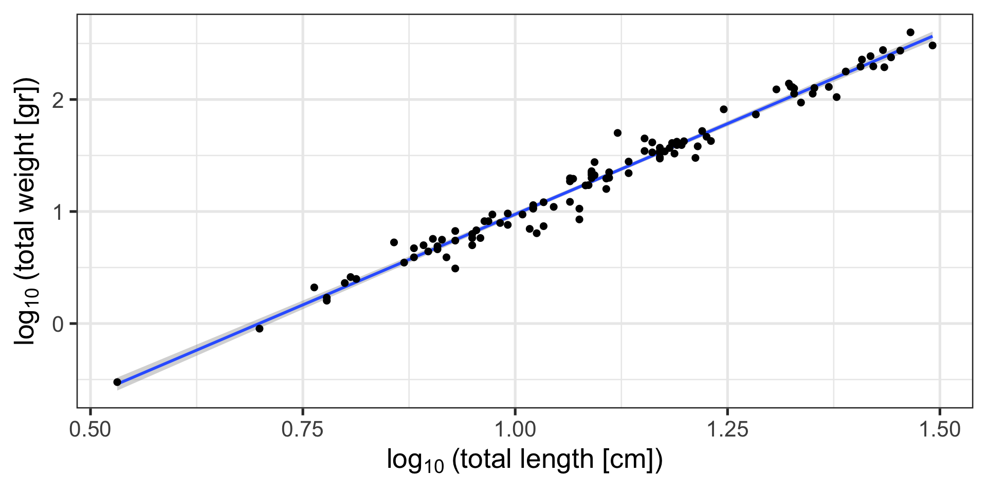
Parenthesis on allometric parameters

Code

library(fixest)
setFixest_dict(c("(Intercept)" = "a",
               "log10(total_length_cm)" = "b",
                "log10(total_weight_gr)" = "Weight"))
feols(log10(total_weight_gr) ~ log10(total_length_cm),
              data = data_lionfish) |> 
  etable()

                feols(log10(tota..
Dependent Var.:             Weight
                                  
a               -2.259*** (0.0544)
b                3.235*** (0.0485)
_______________ __________________
S.E. type                      IID
Observations                   109
R2                         0.97656
Adj. R2                    0.97634
---
Signif. codes: 0 '***' 0.001 '**' 0.01 '*' 0.05 '.' 0.1 ' ' 1

a is my intercept, and indicates the theoretical weight of a fish of length 0 (doesn’t mean much)
b is my slope, and indicates how much log-weight a fish gains for every log-length increase in length
If I know a and b, and I have total_length, I can calculate total_weight

Target

How should these data look like?

How many columns do we want?

What columns names do we want?

We want the data to be “wider”, with 4 columns:

sciname
trophic_level
a
b

The Second Messy Data Again

# A tibble: 15 × 3
   sciname               parameter        value
   <chr>                 <chr>            <dbl>
 1 Pterois volitans      trophic_level  4.4    
 2 Pterois volitans      a             -2.26   
 3 Pterois volitans      b              3.32   
 4 Alloclinus holderi    trophic_level  3.6    
 5 Alloclinus holderi    a              0.0053 
 6 Alloclinus holderi    b              3.08   
 7 Caulolatilus princeps trophic_level  3.6    
 8 Caulolatilus princeps a              0.00708
 9 Caulolatilus princeps b              3.07   
10 Chromis punctipinnis  trophic_level  2.7    
11 Chromis punctipinnis  a              0.0126 
12 Chromis punctipinnis  b              3.03   
13 Embiotoca jacksoni    trophic_level  3.3    
14 Embiotoca jacksoni    a              0.0295 
15 Embiotoca jacksoni    b              2.99

We want to:

Construct new names from the data available in parameter
Use the values from the column value to populate the new columns

Solution: `pivot_wider()`

# Make it tidy
tidy_fish_info <- fish_info |> # Fish info goes into...
  pivot_wider(
    id_cols = sciname,       # The column(s) that specifies my observation
    names_from = parameter,  # My new names will come from...
    values_from = value)     # And my values from...
tidy_fish_info

# A tibble: 5 × 4
  sciname               trophic_level        a     b
  <chr>                         <dbl>    <dbl> <dbl>
1 Pterois volitans                4.4 -2.26     3.32
2 Alloclinus holderi              3.6  0.0053   3.08
3 Caulolatilus princeps           3.6  0.00708  3.07
4 Chromis punctipinnis            2.7  0.0126   3.03
5 Embiotoca jacksoni              3.3  0.0295   2.99

That’s it, pretty straightforward this time

Pivoting arguments

pivot_longer()

cols: Which columns violate the tidy data principle?
names_to: Where should R put the current names of cols?
values_to: Where should R place the data contained by the offending columns?

pivot_wider()

id_cols: Which columns identify my observations?
names_from: Where are the names for my new columns coming from?
values_from: Where are the values for my new variables coming from?

Combining sources of data

left_*, right_*, inner_*, and full_join()

Data Merging: Joins

Why merge data?

You rarely have all the data you need in a single place
Enrich datasets with additional variables

For example: You want to calculate biomass for each of your transects

tidy_kelp has size and abundance, but no information on allometric growth
tidy_fish_info has allometric growth parameters, but no information on size and abundance

We want to add data from tidy_fish_info to tidy_kelp:

For every genus_species in tidy_kelp, we want to get the a and b values in tidy_fish_info as specified by sciname.

Types of joins

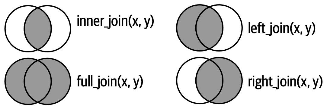
Each circle represents data.frames x and y (or left and right)
The gray area represents the data retained after the operation

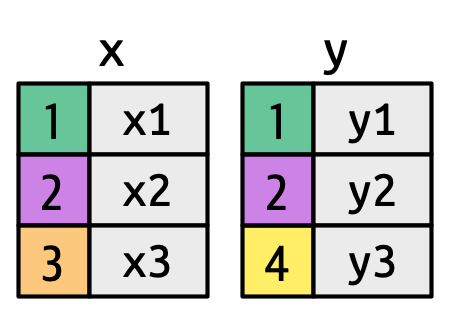
Keys

How does R know what “data overlap” is?
It doesn’t… We need to specify the keys

Remember the data we have

# A tibble: 1,116 × 3
   genus_species         total_length abundance
   <chr>                        <dbl>     <dbl>
 1 Alloclinus holderi             7.5         1
 2 Caulolatilus princeps         17.5         3
 3 Chromis punctipinnis           7.5        14
 4 Embiotoca jacksoni            17.5         6
 5 Embiotoca lateralis           17.5         1
 6 Girella nigricans             22.5         1
 7 Hypsypops rubicundus          17.5         4
 8 Oxyjulis californica           2.5         2
 9 Oxyjulis californica           7.5        61
10 Oxyjulis californica          12.5        46
# ℹ 1,106 more rows

# A tibble: 5 × 4
  sciname               trophic_level        a     b
  <chr>                         <dbl>    <dbl> <dbl>
1 Pterois volitans                4.4 -2.26     3.32
2 Alloclinus holderi              3.6  0.0053   3.08
3 Caulolatilus princeps           3.6  0.00708  3.07
4 Chromis punctipinnis            2.7  0.0126   3.03
5 Embiotoca jacksoni              3.3  0.0295   2.99

Keys are pieces of information to help guide R on how to match the data

What are the keys here?

Target

How should these data look like?

What columns names do we want?

To have columns for a and b on my tidy_kelp data, with at least the following columns:

location
site
transect
genus_species
total_length
abundance
a
b

so that we can calculate total_weight

A `left_join()`

x argument will be tidy_kelp (on the left)
y argument will be tidy_fish_info (on the right)
by argument is where we specify the key (genus_species on the right matches sciname on the left)

Combining data with `left_join()`

left_join(x = tidy_kelp,                                # X is tidy kelp
          y = tidy_fish_info |> select(-trophic_level), # Y is tidy_fish_info, after removing trophic level
          by = join_by(genus_species == sciname))       # And we tell R how to match them

# A tibble: 1,116 × 8
   location site  transect genus_species   total_length abundance        a     b
   <chr>    <chr>    <dbl> <chr>                  <dbl>     <dbl>    <dbl> <dbl>
 1 ASA      North        1 Alloclinus hol…          7.5         1  0.0053   3.08
 2 ASA      North        1 Caulolatilus p…         17.5         3  0.00708  3.07
 3 ASA      North        1 Chromis puncti…          7.5        14  0.0126   3.03
 4 ASA      North        1 Embiotoca jack…         17.5         6  0.0295   2.99
 5 ASA      North        1 Embiotoca late…         17.5         1 NA       NA   
 6 ASA      North        1 Girella nigric…         22.5         1 NA       NA   
 7 ASA      North        1 Hypsypops rubi…         17.5         4 NA       NA   
 8 ASA      North        1 Oxyjulis calif…          2.5         2 NA       NA   
 9 ASA      North        1 Oxyjulis calif…          7.5        61 NA       NA   
10 ASA      North        1 Oxyjulis calif…         12.5        46 NA       NA   
# ℹ 1,106 more rows

Why do I have NAs?
Should I be worried?

Combining data with `right_join()`

right_join(x = tidy_kelp,                                # X is tidy kelp
           y = tidy_fish_info |> select(-trophic_level), # Y is tidy_fish_info, after removing trophic level
           by = join_by(genus_species == sciname))       # And we tell R how to match them

# A tibble: 192 × 8
   location site  transect genus_species    total_length abundance       a     b
   <chr>    <chr>    <dbl> <chr>                   <dbl>     <dbl>   <dbl> <dbl>
 1 ASA      North        1 Alloclinus hold…          7.5         1 0.0053   3.08
 2 ASA      North        1 Caulolatilus pr…         17.5         3 0.00708  3.07
 3 ASA      North        1 Chromis punctip…          7.5        14 0.0126   3.03
 4 ASA      North        1 Embiotoca jacks…         17.5         6 0.0295   2.99
 5 ASA      North        2 Alloclinus hold…          2.5         1 0.0053   3.08
 6 ASA      North        2 Alloclinus hold…          7.5         2 0.0053   3.08
 7 ASA      North        2 Chromis punctip…          2.5         3 0.0126   3.03
 8 ASA      North        2 Chromis punctip…          7.5         6 0.0126   3.03
 9 ASA      North        2 Embiotoca jacks…         17.5         3 0.0295   2.99
10 ASA      North        2 Embiotoca jacks…         27.5         1 0.0295   2.99
# ℹ 182 more rows

What’s different here?

Combining data with `right_join()`

Let’s look at the bottom of the table:

right_join(x = tidy_kelp,                                # X is tidy kelp
           y = tidy_fish_info |> select(-trophic_level), # Y is tidy_fish_info, after removing trophic level
           by = join_by(genus_species == sciname)) |>    # And we tell R how to match them
  tail(10)

# A tibble: 10 × 8
   location site  transect genus_species    total_length abundance       a     b
   <chr>    <chr>    <dbl> <chr>                   <dbl>     <dbl>   <dbl> <dbl>
 1 SSI      North        2 Embiotoca jacks…          7.5         1  0.0295  2.99
 2 SSI      North        2 Embiotoca jacks…         17.5         2  0.0295  2.99
 3 SSI      North        3 Chromis punctip…          7.5        64  0.0126  3.03
 4 SSI      North        3 Embiotoca jacks…         22.5         2  0.0295  2.99
 5 SSI      North        3 Embiotoca jacks…         27.5         1  0.0295  2.99
 6 SSI      South        1 Embiotoca jacks…         17.5         1  0.0295  2.99
 7 SSI      South        1 Embiotoca jacks…         22.5         3  0.0295  2.99
 8 SSI      South        2 Chromis punctip…          7.5        55  0.0126  3.03
 9 SSI      South        2 Embiotoca jacks…         17.5         5  0.0295  2.99
10 <NA>     <NA>        NA Pterois volitans         NA          NA -2.26    3.32

There is no data on the “left” side for lionfish, so there are no matches

Combining data with `inner_join()`

inner_join(x = tidy_kelp,                                # X is tidy kelp
           y = tidy_fish_info |> select(-trophic_level), # Y is tidy_fish_info, after removing trophic level
           by = join_by(genus_species == sciname))       # And we tell R how to match them

# A tibble: 191 × 8
   location site  transect genus_species    total_length abundance       a     b
   <chr>    <chr>    <dbl> <chr>                   <dbl>     <dbl>   <dbl> <dbl>
 1 ASA      North        1 Alloclinus hold…          7.5         1 0.0053   3.08
 2 ASA      North        1 Caulolatilus pr…         17.5         3 0.00708  3.07
 3 ASA      North        1 Chromis punctip…          7.5        14 0.0126   3.03
 4 ASA      North        1 Embiotoca jacks…         17.5         6 0.0295   2.99
 5 ASA      North        2 Alloclinus hold…          2.5         1 0.0053   3.08
 6 ASA      North        2 Alloclinus hold…          7.5         2 0.0053   3.08
 7 ASA      North        2 Chromis punctip…          2.5         3 0.0126   3.03
 8 ASA      North        2 Chromis punctip…          7.5         6 0.0126   3.03
 9 ASA      North        2 Embiotoca jacks…         17.5         3 0.0295   2.99
10 ASA      North        2 Embiotoca jacks…         27.5         1 0.0295   2.99
# ℹ 181 more rows

Combining data with `full_join()`

full_join(x = tidy_kelp,                                # X is tidy kelp
          y = tidy_fish_info |> select(-trophic_level), # Y is tidy_fish_info, after removing trophic level
          by = join_by(genus_species == sciname))       # And we tell R how to match them

# A tibble: 1,117 × 8
   location site  transect genus_species   total_length abundance        a     b
   <chr>    <chr>    <dbl> <chr>                  <dbl>     <dbl>    <dbl> <dbl>
 1 ASA      North        1 Alloclinus hol…          7.5         1  0.0053   3.08
 2 ASA      North        1 Caulolatilus p…         17.5         3  0.00708  3.07
 3 ASA      North        1 Chromis puncti…          7.5        14  0.0126   3.03
 4 ASA      North        1 Embiotoca jack…         17.5         6  0.0295   2.99
 5 ASA      North        1 Embiotoca late…         17.5         1 NA       NA   
 6 ASA      North        1 Girella nigric…         22.5         1 NA       NA   
 7 ASA      North        1 Hypsypops rubi…         17.5         4 NA       NA   
 8 ASA      North        1 Oxyjulis calif…          2.5         2 NA       NA   
 9 ASA      North        1 Oxyjulis calif…          7.5        61 NA       NA   
10 ASA      North        1 Oxyjulis calif…         12.5        46 NA       NA   
# ℹ 1,107 more rows

Potential pitfalls

duplicate keys, keys not fully specified

Example: keys not fully specified

# A tibble: 10 × 5
   sciname               trophic_level        a     b north_south
   <chr>                         <dbl>    <dbl> <dbl> <chr>      
 1 Pterois volitans                4.4 -2.48     3.66 North      
 2 Pterois volitans                4.4 -2.26     3.32 South      
 3 Alloclinus holderi              3.6  0.00583  3.39 North      
 4 Alloclinus holderi              3.6  0.0053   3.08 South      
 5 Caulolatilus princeps           3.6  0.00779  3.38 North      
 6 Caulolatilus princeps           3.6  0.00708  3.07 South      
 7 Chromis punctipinnis            2.7  0.0138   3.33 North      
 8 Chromis punctipinnis            2.7  0.0126   3.03 South      
 9 Embiotoca jacksoni              3.3  0.0325   3.29 North      
10 Embiotoca jacksoni              3.3  0.0295   2.99 South

Failing to specify keys results in duplicates

tidy_kelp |> # Tidy kelp goes into... (Yes, you can pipe)
  left_join(tidy_fish_info2 |> select(-trophic_level),
            by = join_by(genus_species == sciname)) # I failed to link site to north_south

Warning in left_join(tidy_kelp, select(tidy_fish_info2, -trophic_level), : Detected an unexpected many-to-many relationship between `x` and `y`.
ℹ Row 1 of `x` matches multiple rows in `y`.
ℹ Row 3 of `y` matches multiple rows in `x`.
ℹ If a many-to-many relationship is expected, set `relationship =
  "many-to-many"` to silence this warning.

# A tibble: 1,307 × 9
   location site  transect genus_species   total_length abundance        a     b
   <chr>    <chr>    <dbl> <chr>                  <dbl>     <dbl>    <dbl> <dbl>
 1 ASA      North        1 Alloclinus hol…          7.5         1  0.00583  3.39
 2 ASA      North        1 Alloclinus hol…          7.5         1  0.0053   3.08
 3 ASA      North        1 Caulolatilus p…         17.5         3  0.00779  3.38
 4 ASA      North        1 Caulolatilus p…         17.5         3  0.00708  3.07
 5 ASA      North        1 Chromis puncti…          7.5        14  0.0138   3.33
 6 ASA      North        1 Chromis puncti…          7.5        14  0.0126   3.03
 7 ASA      North        1 Embiotoca jack…         17.5         6  0.0325   3.29
 8 ASA      North        1 Embiotoca jack…         17.5         6  0.0295   2.99
 9 ASA      North        1 Embiotoca late…         17.5         1 NA       NA   
10 ASA      North        1 Girella nigric…         22.5         1 NA       NA   
# ℹ 1,297 more rows
# ℹ 1 more variable: north_south <chr>

Correctly specify the two keys

tidy_kelp |> # Tidy kelp goes into... (Yes, you can pipe)
  left_join(tidy_fish_info2 |> select(-trophic_level),
            by = join_by(genus_species == sciname,
                         site == north_south))

# A tibble: 1,116 × 8
   location site  transect genus_species   total_length abundance        a     b
   <chr>    <chr>    <dbl> <chr>                  <dbl>     <dbl>    <dbl> <dbl>
 1 ASA      North        1 Alloclinus hol…          7.5         1  0.00583  3.39
 2 ASA      North        1 Caulolatilus p…         17.5         3  0.00779  3.38
 3 ASA      North        1 Chromis puncti…          7.5        14  0.0138   3.33
 4 ASA      North        1 Embiotoca jack…         17.5         6  0.0325   3.29
 5 ASA      North        1 Embiotoca late…         17.5         1 NA       NA   
 6 ASA      North        1 Girella nigric…         22.5         1 NA       NA   
 7 ASA      North        1 Hypsypops rubi…         17.5         4 NA       NA   
 8 ASA      North        1 Oxyjulis calif…          2.5         2 NA       NA   
 9 ASA      North        1 Oxyjulis calif…          7.5        61 NA       NA   
10 ASA      North        1 Oxyjulis calif…         12.5        46 NA       NA   
# ℹ 1,106 more rows

Full pipeline to get biomass

# Tidy the transect data
tidy_kelp <- data_kelp |> # data_kelp goes into...
  pivot_longer(
    cols = starts_with("TL_"), #specify columns to pivot
    names_to = "total_length", # Where should column names be placed?
    values_to = "abundance",   # Where should values be placed?
    values_drop_na = TRUE,     # Specify that NA values should be removed)
    names_prefix = "TL_") |>   # Remove "TL_" from the total length
  mutate(total_length = as.numeric(total_length) -2.5) # Use mutate to rewrite column

# Tidy the allometric data data
tidy_fish_info <- fish_info |> # Fish info goes into...
  pivot_wider(
    id_cols = sciname,       # The column(s) that specifies my observation
    names_from = parameter,  # My new names will come from...
    values_from = value) |>  # And my values from...
  select(-trophic_level)

# And now combine them
biomass <-tidy_kelp |> 
  left_join(tidy_fish_info,
            by = join_by(genus_species == sciname)) |>
 # And use last week's knowledge to calculate the rest
  mutate(biomass = (a * total_length ^ b) * abundance / 1000 ) |> 
  group_by(location, site, transect) |> 
  summarize(biomass = sum(biomass, na.rm = T) / 60)

# A tibble: 82 × 4
# Groups:   location, site [28]
   location site  transect  biomass
   <chr>    <chr>    <dbl>    <dbl>
 1 ASA      North        1 0.0190  
 2 ASA      North        2 0.0182  
 3 ASA      North        3 0.0217  
 4 ASA      South        1 0       
 5 ASA      South        2 0.0132  
 6 ASA      South        3 0.188   
 7 BMA      North        1 0.0137  
 8 BMA      North        2 0.0245  
 9 BMA      North        3 0.000188
10 BMA      South        1 0.0144  
# ℹ 72 more rows

Best Practices

Data Tidying:

Start with the end in mind - what do you want your data to look like?
Use pivot_longer() when column names are values
Use pivot_wider() when observations are scattered across rows
Check for data consistency after pivoting

Joining Data:

Always specify the by argument explicitly
Check for duplicate keys before joining
Use left_join() as default unless you have a specific reason
Validate results after joining

Wickham, Hadley. 2014. “Tidy Data.” The Journal of Statistical Software 59. http://www.jstatsoft.org/v59/i10/.

Wickham, Hadley, Mine Cetinkaya-Rundel, and Garrett Grolemund. 2023. R for Data Science: Import, Tidy, Transform, Visualize, and Model Data. 2nd ed. Sebastopol, CA: O’Reilly Media.

EVR 628- Intro to Environmental Data Science

Learning Objectives

Tidy Data

Messy Data?

The {tidyr} Package

Changing shape of data

1) Lengthening data

Target

The Messy Data Again

Solution: pivot_longer()

Dealing with NAs

Removing the prefix

Making total_length numeric

Other arguments to pivot_longer()

2) Widening data

Parenthesis on allometric parameters

Target

The Second Messy Data Again

Solution: pivot_wider()

Pivoting arguments

Combining sources of data

Data Merging: Joins

Types of joins

Keys

Target

A left_join()

Combining data with left_join()

Combining data with right_join()

Combining data with right_join()

Combining data with inner_join()

Combining data with full_join()

Potential pitfalls

Example: keys not fully specified

Failing to specify keys results in duplicates

Correctly specify the two keys

Full pipeline to get biomass

Best Practices

The `{tidyr}` Package

Solution: `pivot_longer()`

Making `total_length` numeric

Other arguments to `pivot_longer()`

Solution: `pivot_wider()`

A `left_join()`

Combining data with `left_join()`

Combining data with `right_join()`

Combining data with `right_join()`

Combining data with `inner_join()`

Combining data with `full_join()`