# Shark analysis
lengths <- c(6, 4.1, 2.8, 5.5, 3.9, 5.8)
sharks <- c("Great White Shark", "Lemon Shark", "Bull Shark", "Hammerhead Shark", "Mako Shark", "Great White Shark")
shark_data <- data.frame(
  lengths,
  sharks
)
shark_data$sharks[shark_data$length == max(shark_data$length)]
[1] "Great White Shark"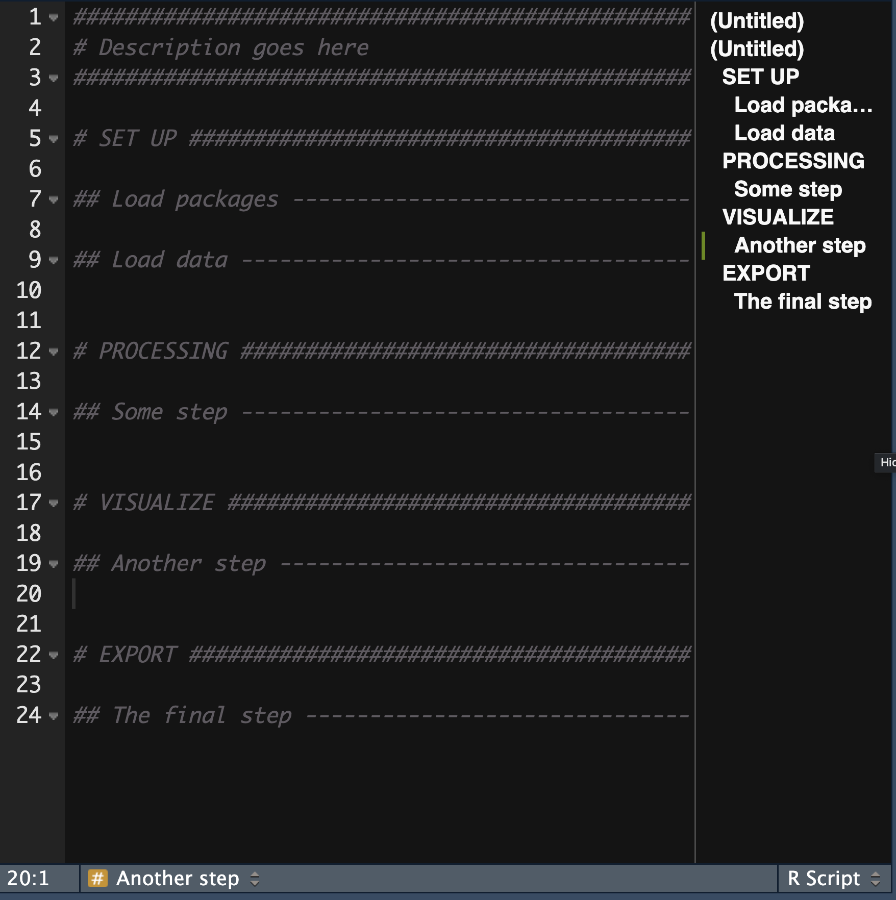


Comments
Text embedded within your script for humans to read
Helps other people (including future you) understand what’s going on
We use the
#sign to prevent the computer from reading it