Working with spatial data in R: Raster

Today’s analysis

Preamble

Rice’s whale (Balaenoptera ricei) are a relatively new species discovered in our backyard. Their distribution is limited to the Gulf, and some have raised concerns about potential interactions with fishing gear for two reasons:

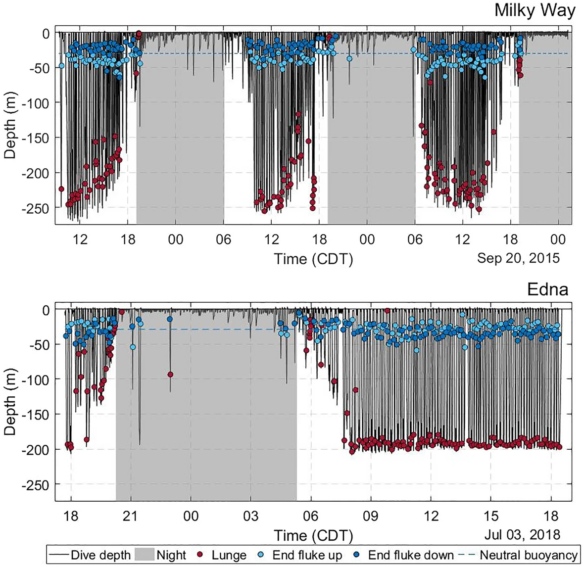
1. Rice’s whales sleep near the surface, which exposes them to early boat traffic (see figure below).
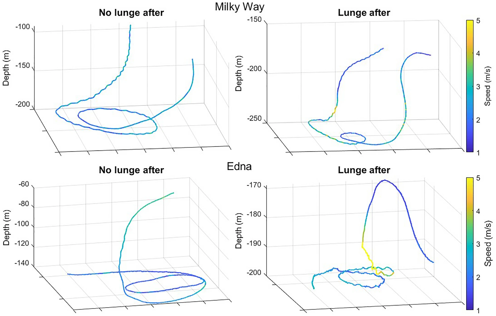
2. When Rice’s whales feed, they are thought to perform circling movements with the bottom. These could expose them to interactions with bottom set gear (see figure below).

Rice’s whale sleep near the surface. Source: Kok et al. (2023)

Rice’s whale exhibit circling behavior near the bottom. Source: Kok et al. (2023)

The task at hand

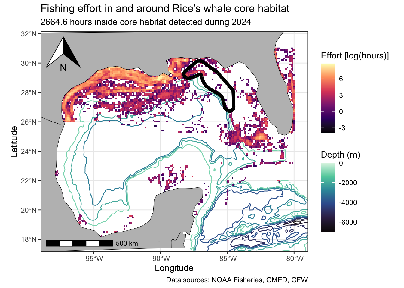
NOAA Fisheries has identified Rice’s whale core habitat. You have access to spatially-explicit fishing effort data for 2024 (via EVR628tools::data_fishing_effort). Your tasks are to measure the amount of fishing effort ocurring within Rice’s whale core habitat and produce a map.

Part 1: Set up

Exercise 1: Download datasets

Post-it up

Rice’s whale Core Habitat

1. Go to NOAA Fisheries and download the Shapefile for Rice’s Whale Core Distribution Area.
2. You will be prompted to download a zipped folder. Save it to your data/raw folder in the EVR_628 project.
3. Unzip / extract it like we did before¹
4. Is this a vector or raster file?

Depth

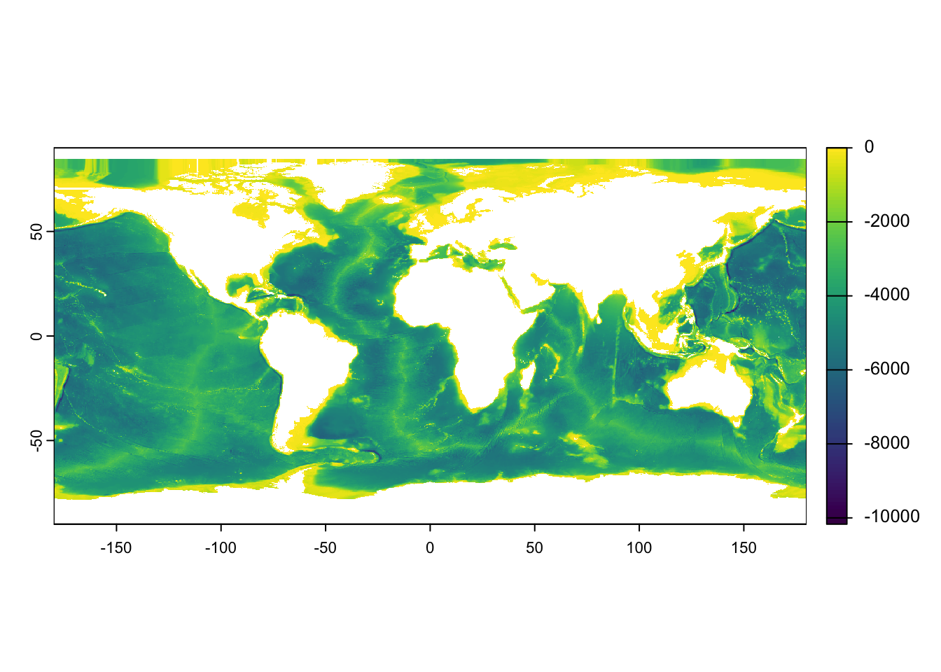
1. Click here to download a global raster for depth.²
2. Save it to data/raw
3. Is this a vector or a raster file?

Post-it down

Exercise 2: Read datasets into R

Post-it up

1. Create a new R script called rices_whale.R and save it to your scripts/analysis folder.
2. Add a basic comment structure to your script.
3. Load all the packages that we will need: EVR628tools, ggspatial, rnaturalearth, tidyverse, sf, terra, tidyterra, and mapview.
4. You will now create three objects:
   • whale <-: Use read_sf() to load Rice’s whale core habitat vector. Note: you don’t need to list every file; simply list the path to the .shp file.
   • depth <-: Use rast() to load the depth raster.
   • coast <-: Use ne_countries() to load vector data for U.S.A, Mexico, Belize, and Guatemala³.
5. Use data() to load the data_fishing_effort dataset from the EVR628tools package.
6. Quickly inspect your whale and coast data using mapview(). Inspect depth with plot().

Post-it down

# Load packages ----------------------------------------------------------------
library(EVR628tools)   # For fishing effort data and color palettes
library(ggspatial)     # To add map elements to a ggplot
library(rnaturalearth) # To add country outlines
library(tidyverse)     # General data wrangling
library(sf)            # Working with vector data
library(terra)         # Working with raster data
library(tidyterra)     # Working with raster data in tidy approach
library(mapview)       # To quickly inspect data

# Load data --------------------------------------------------------------------
# Load whale core habitat
whale <- read_sf("data/raw/shapefile_Rices_whale_core_distribution_area_Jun19_SERO/shapefile_Rices_whale_core_distribution_area_Jun19_SERO.shp")
# Load depth raster
depth <- rast("data/raw/depth_raster.tif")
# Load world's coastline
coast <- ne_countries(country = c("United States of America", "Mexico", "Belize", "Guatemala"))
# Load fishing effort data.frame
data("data_fishing_effort")

# Quick inspections
mapview(list(whale, coast))

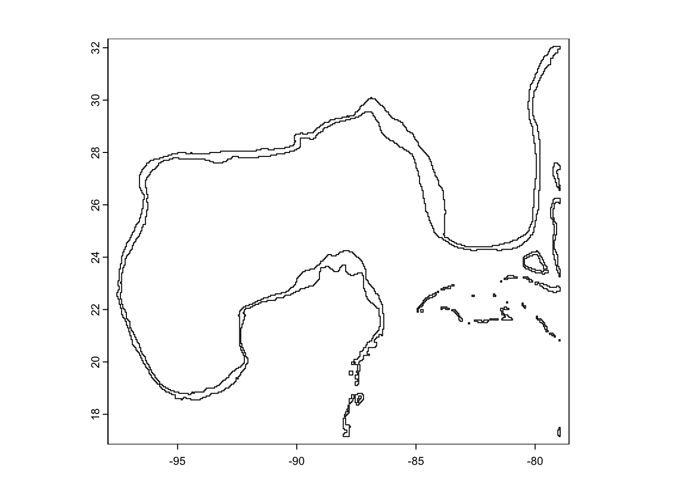
plot(depth)

Part 2: Data wrangling

Exercise 1: Rasterize fishing effort

Printing the data_fishing_effort object reveals that it contains monthly fishing effort by pixel⁴, but it is not yet a raster object… we’ll get there after some piping.

Post-it up

1. Look at the documentation for the ?rast() function. Scroll down to where it says “## S4 method for signature 'data.frame'”.
2. Start building a pipeline. Create a new object called effort_raster <- that receives the data_fishing_effort object.
3. Calculate total fishing effort (in hours) for each pixel (lon, lat) using group_by() and summarize(). Name the new column hours.

Post-it down

4. After the summarize(), pipe into rast(). For the crs argument, use crs = "EPSG:4326"⁵.
5. Print the new effort_raster to your console.
   • What is the class of effort_raster?
   • What is the res of effort_raster?
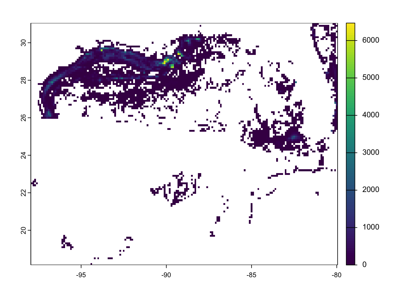
6. Make a quick plot of your new raster object.

# Create a new object to contain a raster of fishing effort
effort_raster <- data_fishing_effort |>    # Start with my data.frame
  group_by(lon, lat) |>                    # group by lon and lat
  summarize(hours = sum(effort_hours)) |>  # Calculate total effort by pixel
  rast(crs = "EPSG:4326")                  # Build a raster

# Print raster to console
effort_raster

class       : SpatRaster 
size        : 129, 180, 1  (nrow, ncol, nlyr)
resolution  : 0.1, 0.1  (x, y)
extent      : -97.95, -79.95, 18.15, 31.05  (xmin, xmax, ymin, ymax)
coord. ref. : lon/lat WGS 84 (EPSG:4326) 
source(s)   : memory
name        :   hours 
min value   :    0.00 
max value   : 6468.06 

# Quick plot of my raster
plot(effort_raster)

Exercise 2: Calculate total fishing in core habitat

We now want to extract the data associated with pixels inside the whale’s core habitat.

We’ll do this one together.

1. Look at the documentation for the ?extract() function in the terra package.
2. Pay attention to the section “## S4 method for signature 'SpatRaster,SpatVector'”
   • What are x and y?
   • What does the fun argument do?
   • What is the exact parameter for?
3. Extract all fishing effort occurring inside the whale’s core habitat. Use fun = sum and na.rm = T
4. Then try adding touches = T. What happens to the answer?
5. Now use exact = T. What happens now?

# extract(effort_raster, whale)                      # Simple extraction (I'm not running it here to save space)
extract(effort_raster, whale, fun = sum, na.rm = T)  # Calculate sum

  ID   hours
1  1 2691.67

extract(effort_raster, whale, fun = sum, na.rm = T, touches = T) # Keep all pixels touched by the raster

  ID   hours
1  1 2815.58

extract(effort_raster, whale, fun = sum, na.rm = T, exact = T) # Calculate the weighted sum

  ID    hours
1  1 2664.666

Exercise 3: Prepare layers for plotting

We’ll do this one together.

1. What is the extent of the depth raster? How about the extent dor the coast vector? Clearly we will need to modify their extents.
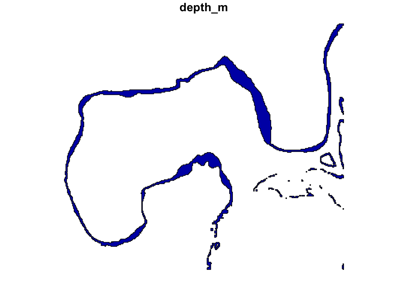
2. Use crop() to crop the depth raster so that it matches the extent of the effort_raster⁶. Save the new depth raster to gulf_depth.
3. The coast vector data contains the entire boundaries for the four countries. Let’s also crop it to match effort_raster, but this time using st_crop(). Save the new vector file to gulf_coast.

gulf_depth <- crop(depth, extend(effort_raster, 10))
gulf_coast <- st_crop(coast, extend(effort_raster, 10))

Part 3: Visualize

Exercise 1: Build a map

Let’s replicate the map below.

 # Start a plot
ggplot() +
  # Add the depth contours as the first laeyer
  geom_spatraster_contour(data = gulf_depth,
                          aes(colour = after_stat(level)),
                          linewidth = 0.5) +
  # Add fishing effort raster on top
  geom_spatraster(data = log(effort_raster)) +
  # Add gulf coast coastline
  geom_sf(data = gulf_coast,
          fill = "gray",
          color = "black") +
  # Add whale's core habitat
  geom_sf(data = whale, fill = "transparent",
          color = "black",
          linewidth = 2) +
  # Modify the colors for the depth contours
  scale_color_viridis_c(option = "mako") +
  # Modify the fill of the effort raster
  scale_fill_viridis_c(option = "magma",
                       na.value = "transparent") +
  # Modify the theme
  theme_bw() +
  # Add a north arrow from ggspatial
  annotation_north_arrow(location = "tl") +
  # Add a scalebar from ggspatial
  annotation_scale(location = "bl") +
  # Trim whitespace
  scale_x_continuous(expand = c(0, 0)) +
  scale_y_continuous(expand = c(0, 0)) +
  # Update labels
  labs(color = "Depth (m)",
       fill = "Effort [log(hours)]",
       x = "Longitude",
       y = "Latitude",
       title = "Fishing effort in and around Rice's whale core habitat",
       subtitle = "2664.6 hours inside core habitat detected during 2024",
       caption = "Data sources: NOAA Fisheries, GMED, GFW")

Extra

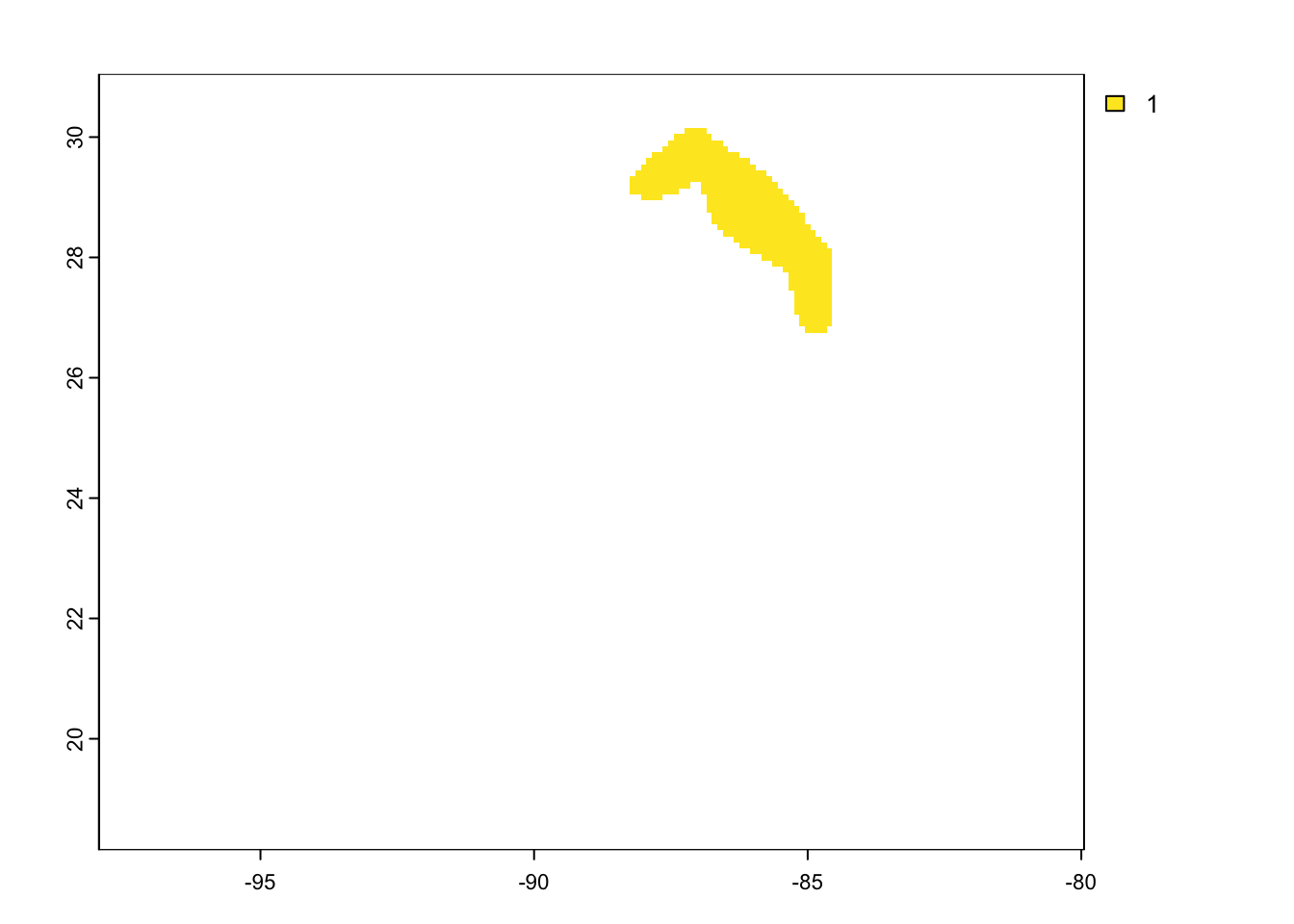
Rasterize a vector

Our exercises above had us take point data on a regular grid and convert them to a raster object. But what if we wanted to start with a spatial vector file? The chunk below takes the whale’s core habitat and produces a raster version of it. The key function is rasterize().

whale_raster <- rasterize(whale, effort_raster)
plot(whale_raster)

Vectorize a raster

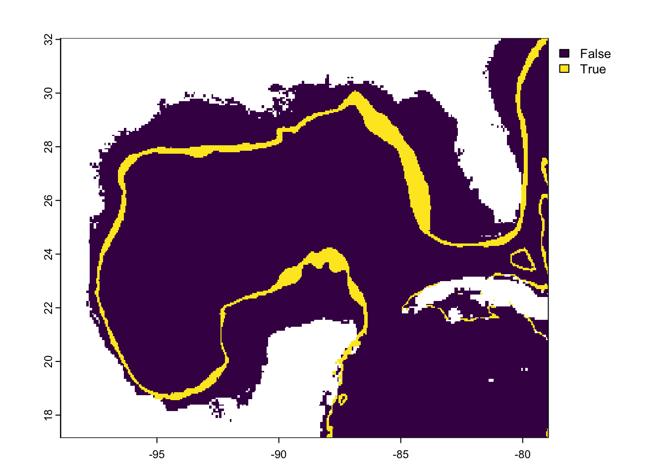
What about the opposite case? We might have raster data outlining, say, areas between 100–400 m deep (Rice’s whale depth range as reported by NOAA.)

# Create a raster of depths that are relevant
range_rast <- (gulf_depth > -400) & (gulf_depth < -100)
plot(range_rast)

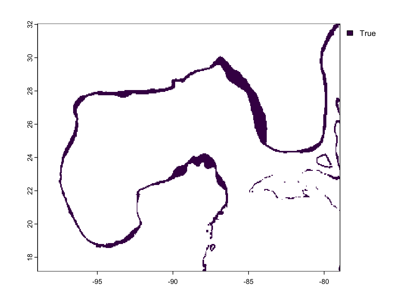
# Anything outside the range is now NA
range_rast[!range_rast] <- NA
plot(range_rast)

# Polygonize the outline
range_vect <- as.polygons(range_rast, dissolve = T)
plot(range_vect)

# Convert it to an sf object
range_vect <- as.polygons(range_rast, dissolve = T) |> 
  st_as_sf()
plot(range_vect)

References

Kok, Annebelle C M, Maya J Hildebrand, Maria MacArdle, Anthony Martinez, Lance P Garrison, Melissa S Soldevilla, and John A Hildebrand. 2023. “Kinematics and Energetics of Foraging Behavior in Rice’s Whales of the Gulf of Mexico.” Sci. Rep. 13 (June): 8996.

Footnotes

1. Mac users double click on the zip folder. Windows users use the “Extract” or “Unzip” button in your toolbar.

2. The data come from GMED: Global Marine Environment Datasets for environment visualization and species distribution modelling, but UM’s firewall doesn’t allow access.

3. Hint: You will need to use country = c("United States of America", "Mexico", "Belize", "Guatemala")

4. Hint: Use ?data_fishing_effort to look at the documentation

5. More on EPSG codes at EPSG.io

6. Hint: You can also use extend() as raster version of the st_buffer() that I used on Tuesday