Working with spatial data in R: Vector

Author

Juan Carlos Villaseñor-Derbez (JC)

Exercise 0 - Set up

Open your EVR628 R project
Install / update the packages as needed using the code below:

install.packages("sf")            # You should have this from Tuesday
install.packages("rnaturalearth") # You should have this from Tuesday
install.packages("mapview")       # You should have this from Tuesday
remotes::install_github("jcvdav/EVR628tools")

Start a new R script called vector_data.R and save it under scripts/02_analysis.R
Add a code header
Load the tidyverse, janitor, sf, rnaturalearth, mapview, and EVR628tools

Exercise 1 - Inspecting spatial data

Part 1: FL counties

Post-it up

Go to the FDOT website and download the county Geopackage file¹. Make sure you save them to your data/raw folder.
Look at the documentation for ?read_sf
Read the FL counties geopackage and assign it to an object called FL_counties <-
Immediately after that, pipe into clean_names() and then again into st_set_geometry("geometry"). FDOT data are weird, I will explain why we are doing this.

Post-it down

Code

# Load packages
library(tidyverse)
library(janitor)
library(sf)
library(rnaturalearth)
library(mapview)
library(EVR628tools)

# Load FL counties
FL_counties <- read_sf("data/raw/Florida_County_Boundaries_with_FDOT_Districts_-801746881308969010.gpkg") |> 
  clean_names() |> 
  st_set_geometry("geometry")

Warning in CPL_read_ogr(dsn, layer, query, as.character(options), quiet, : GDAL
Message 1: Non-conformant content for record 1 in column CreationDate,
2025-10-07T20:05:32.0Z, successfully parsed

Part 2: Inspect FL counties

Post-it up

How many columns do we have? How many rows?
What are the column names?
Use R’s base plot() to visualize them. CAREFUL, make sure you specify max.plot = 1.
Now use mapview to visualize your data.

Post-it down

Code

# Inspect attributes
dim(FL_counties)

[1] 67 16

Code

colnames(FL_counties)

 [1] "name"             "first_fips"       "objectid_1"       "fdot_distr"      
 [5] "district_string"  "depcode"          "depcodenum"       "d_code"          
 [9] "county"           "fdot_county_code" "global_id"        "creation_date"   
[13] "creator"          "edit_date"        "editor"           "geometry"

Code

# Base plot
plot(FL_counties, max.plot = 1)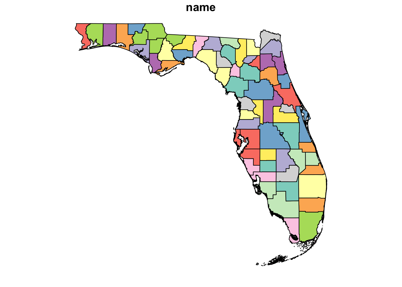

Code

# Mapview
mapview(FL_counties)

Part 3: Prep the data

Post-it up

The FL County vector file has more columns than we need. Modify your pipeline to retain only county name and first_fips (rename them as county_name and county_fips).
Load the new data_hurricanes data that I’ve included in the latest version of the EVR628tools package
Quickly inspect them with the usual methods

Post-it down

Code

FL_counties <- read_sf("data/raw/Florida_County_Boundaries_with_FDOT_Districts_-801746881308969010.gpkg") |> 
  clean_names() |> 
  st_set_geometry("geometry") |> 
  select(county_name = name,
         county_fips = first_fips)

Warning in CPL_read_ogr(dsn, layer, query, as.character(options), quiet, : GDAL
Message 1: Non-conformant content for record 1 in column CreationDate,
2025-10-07T20:05:32.0Z, successfully parsed

Code

data("data_hurricanes")

dim(data_hurricanes)

[1] 51  4

Code

# Ignore the if statement, this is just a workaround for myself
mapview(data_hurricanes)

Exercise 2 - Spatial operations

Part 1: Spatial join (`st_join`)

Task: Count the number of storms to which each county has been exposed between 2022 and 2024

We’ll do this one together

Look at the documentation for the ?st_join() function
Let’s create a new object called county_hur <- that will contain the outcome of the join operation
Now lets count the number of storms per county
Let’s make a map, where the fill of each county is given by the number of storms

Code

county_hur <- st_join(FL_counties, data_hurricanes) |> 
  group_by(county_name, county_fips) |> 
  summarize(n_storms = n_distinct(name,
                                  na.rm = T))

`summarise()` has grouped output by 'county_name'. You can override using the
`.groups` argument.

Code

ggplot() +
  geom_sf(data = county_hur,
          mapping = aes(fill = n_storms)) +
  theme_minimal()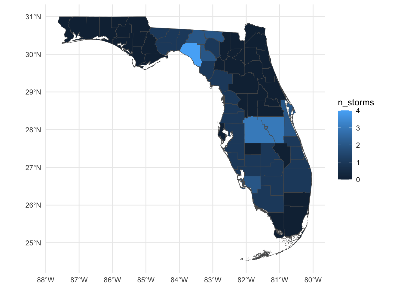

Part 2: Spatial filter (`st_filter`)

Task: Which hurricanes affected FL counties?

Post-it up

Read the documentation for the ?st_filter() function
If our goal is to filter hurricanes based on their location, what is x and what is y?
Use the st_filter() function to find the hurricanes that went over FL counties, save the output to FL_hurricanes
Make a quick map using ggplot
Look at the documentation for st_crop()
Extend your pipeline for FL_hurricanes to use st_crop()

Post-it down

Code

FL_hurricanes <- st_filter(data_hurricanes, FL_counties) |> 
  st_crop(FL_counties)

Warning: attribute variables are assumed to be spatially constant throughout
all geometries

Code

ggplot() +
  geom_sf(data = FL_hurricanes,
          mapping = aes(color = name)) +
  theme_minimal()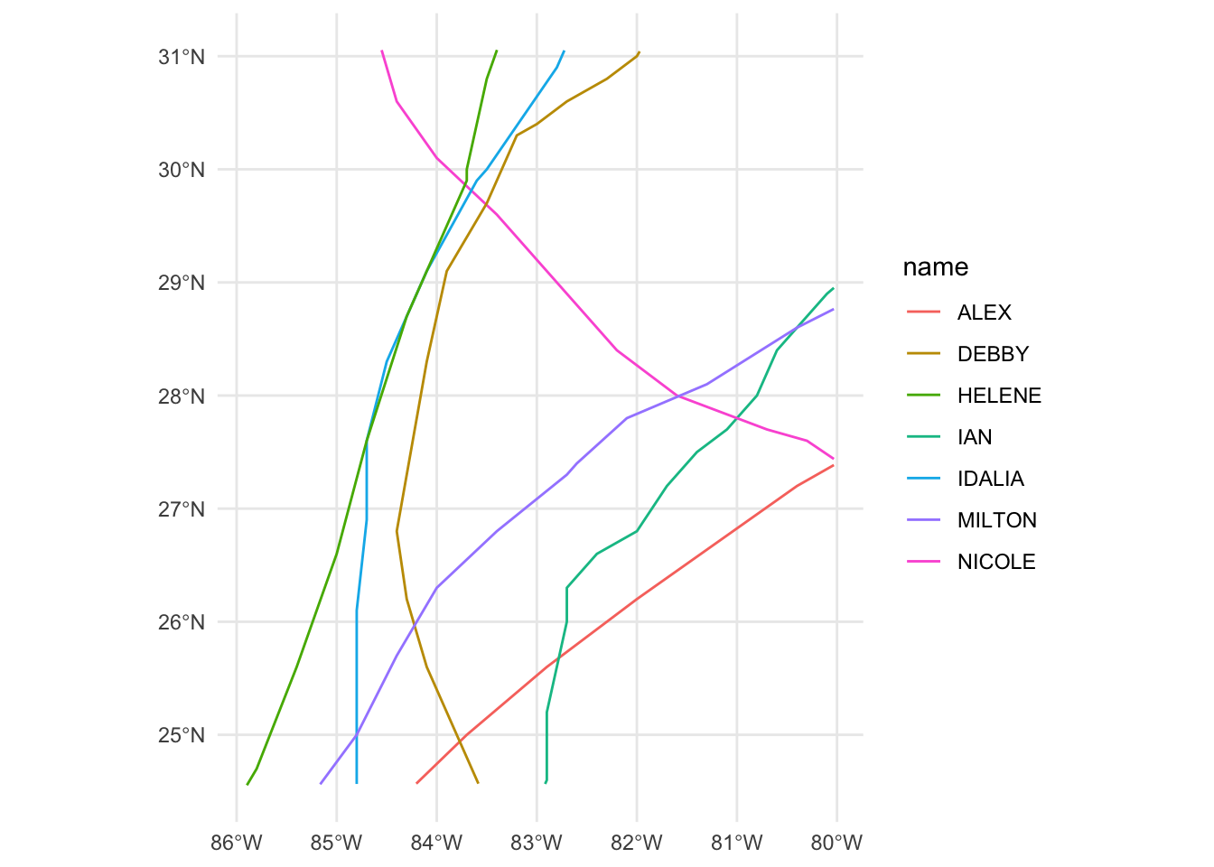

Part 3: Final map

Replicate the map below

Code

ggplot() +
  geom_sf(data = county_hur,
          mapping = aes(fill = n_storms),
          color = "black") + 
  geom_sf(data = FL_hurricanes,
          mapping = aes(color = name)) +
  scale_fill_viridis_c() +
  scale_color_manual(values = palette_UM(n = 7)) +
  theme_bw() +
  labs(title = "Storm exposure by county",
       subtitle = "Named storms between 2022 and 2024",
       x = "Lon",
       y = "Lat",
       color = "Storm name",
       fill = "# Storms")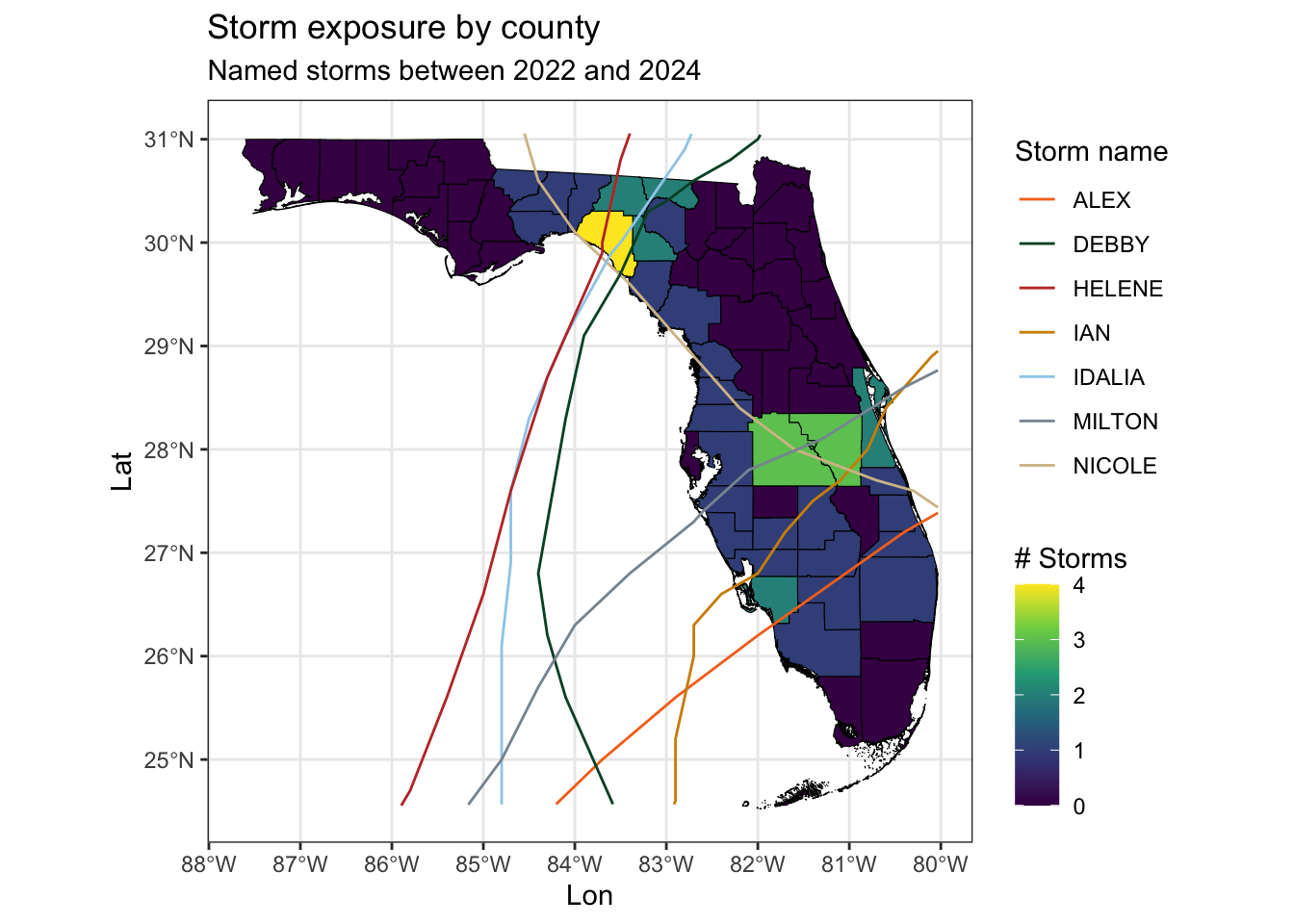

Exercise 3 - Building your own `sf` object

Post-it up

Load the data_milton dataset from the EVR628tools package into your environment and familiarize yourself with it (again)
Look at the documentation for ?st_as_sf()
Convert our data_milton data.frame into an sf object called milton_sf
Plot them using base plot()

Post-it down

Code

data("data_milton")

head(data_milton, 10)

# A tibble: 10 × 7
   name   iso_time              lat   lon wind_speed pressure sshs 
   <chr>  <dttm>              <dbl> <dbl>      <dbl>    <dbl> <chr>
 1 MILTON 2024-10-04 18:00:00  21   -94.6         30     1009 -3   
 2 MILTON 2024-10-04 21:00:00  20.8 -94.9         30     1009 -3   
 3 MILTON 2024-10-05 00:00:00  20.8 -95.2         30     1008 -3   
 4 MILTON 2024-10-05 03:00:00  21   -95.3         30     1008 -3   
 5 MILTON 2024-10-05 06:00:00  21.4 -95.4         30     1008 -3   
 6 MILTON 2024-10-05 09:00:00  21.7 -95.5         30     1008 -3   
 7 MILTON 2024-10-05 12:00:00  22   -95.5         30     1008 -1   
 8 MILTON 2024-10-05 15:00:00  22.3 -95.5         33     1007 -1   
 9 MILTON 2024-10-05 18:00:00  22.5 -95.5         35     1006 0    
10 MILTON 2024-10-05 21:00:00  22.6 -95.5         35     1005 0

Code

# Convert to sf object
milton_sf <- st_as_sf(data_milton,
                      coords = c("lon", "lat"),
                      crs = "EPSG:4326")

# Plot them
plot(milton_sf, max.plot = 1)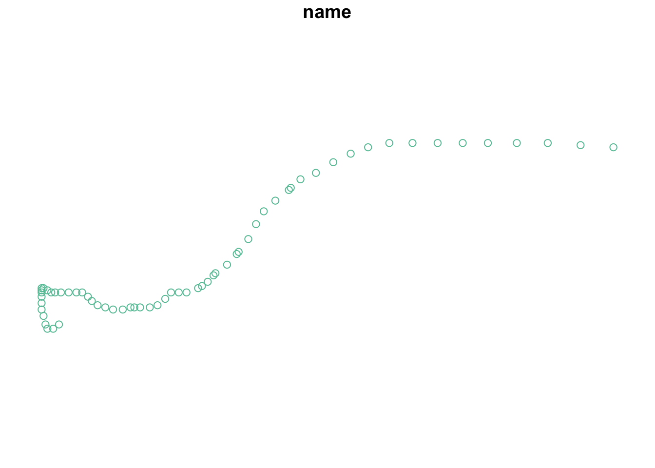

Additional exercises

1) Converting points to linestrings

Take the milton_sf data and convert the points into a track (so, from POINT to LINESTRING)

Code

nrow(milton_sf) # One row per point

[1] 62

Code

milton_sf_track <- milton_sf |> 
  # I need to specify the groups, even though there's only one
  group_by(name) |>              
  summarize(do_union = FALSE,
            .groups = "drop")

nrow(milton_sf_track) # One row per group, but still as points in a MULTIPOINT geometry

[1] 1

Code

st_geometry_type(milton_sf_track)

[1] MULTIPOINT
18 Levels: GEOMETRY POINT LINESTRING POLYGON MULTIPOINT ... TRIANGLE

Code

ggplot(milton_sf_track) +
  geom_sf()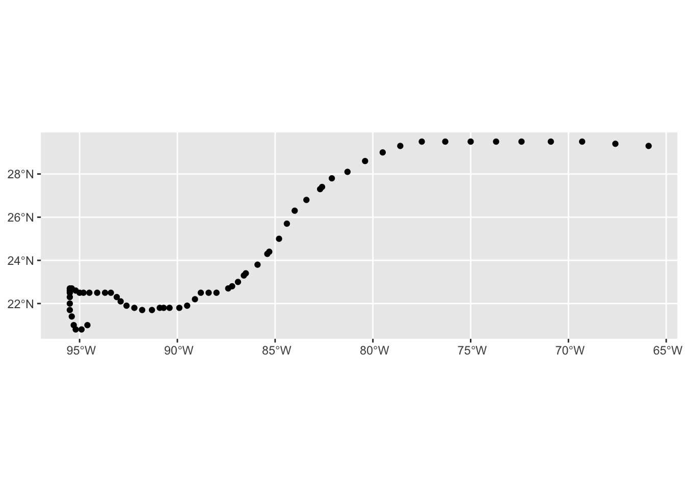

Code

# After the summarize, all points are individually combined as a MULTIPOINT object,
# so we need to convert them to a LINESTRING. The full pipeline looks like this:
milton_sf_track <- milton_sf |> 
  group_by(name) |>
  summarize(do_union = FALSE,
            .groups = "drop") |> 
  st_cast("LINESTRING")           

nrow(milton_sf_track) # One row per group, but now as a LINESTRING

[1] 1

Code

st_geometry_type(milton_sf_track)

[1] LINESTRING
18 Levels: GEOMETRY POINT LINESTRING POLYGON MULTIPOINT ... TRIANGLE

Code

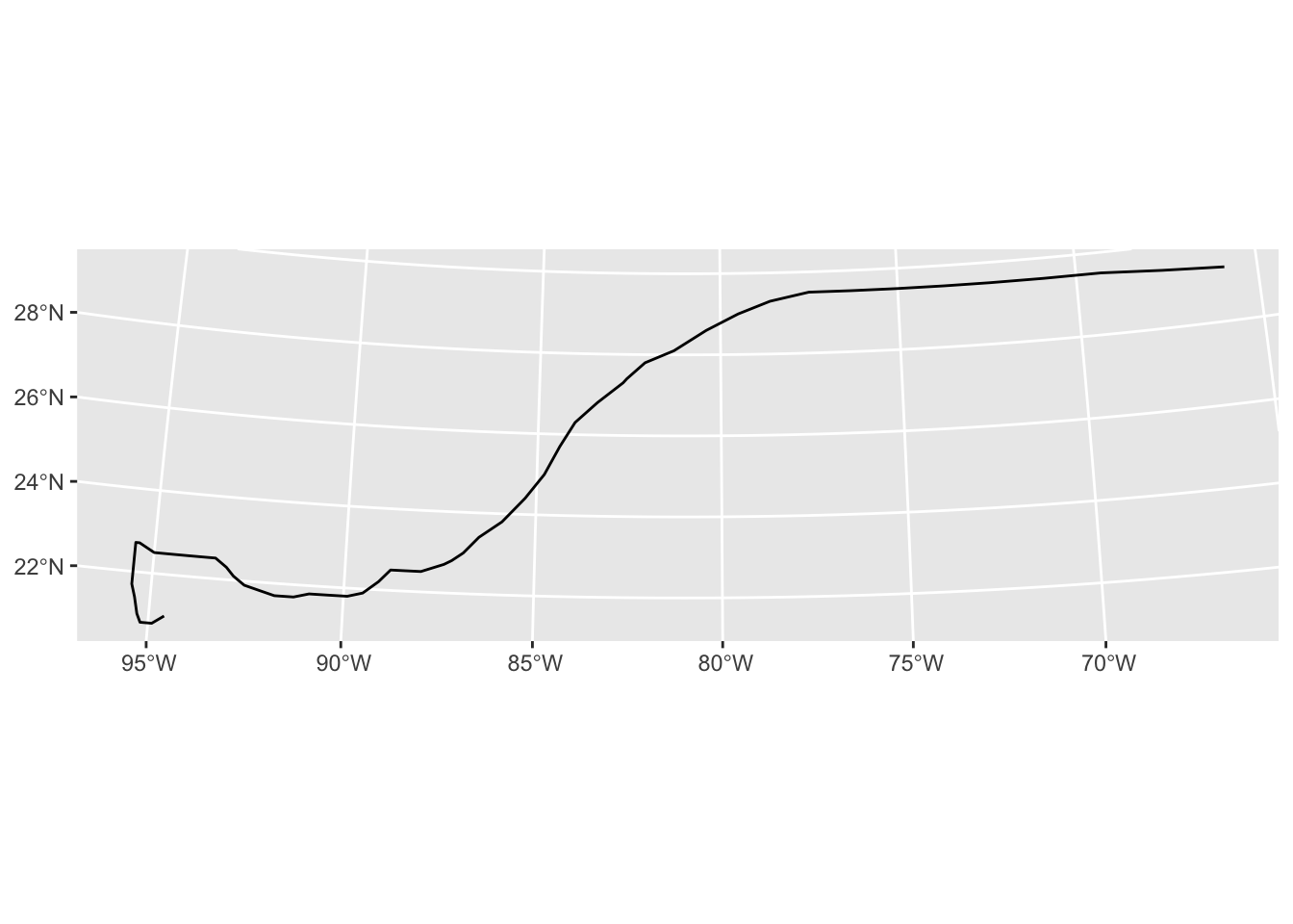
ggplot(milton_sf_track) +
  geom_sf()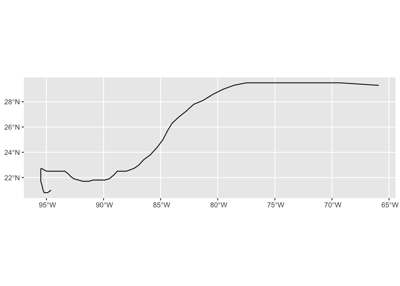

2) Reproject the data to a different CRS

Take the new milton_sf_track and project it to UTM zone 16N. epsg.io tells us the EPSG code is EPSG:26917-1714. After reprojecting, look at the difference in shape relative to the figure above.

Code

milton_sf_track_UTM <- st_transform(milton_sf_track, crs = "EPSG:26917-1714")

ggplot(milton_sf_track_UTM) + 
         geom_sf()

Footnotes

Geopackage are superior to shapefiles or GeoJSON files ↩︎

Exercise 0 - Set up

Exercise 1 - Inspecting spatial data

Part 1: FL counties

Part 2: Inspect FL counties

Part 3: Prep the data

Exercise 2 - Spatial operations

Part 1: Spatial join (st_join)

Part 2: Spatial filter (st_filter)

Part 3: Final map

Exercise 3 - Building your own sf object

Additional exercises

1) Converting points to linestrings

2) Reproject the data to a different CRS

Footnotes

Part 1: Spatial join (`st_join`)

Part 2: Spatial filter (`st_filter`)

Exercise 3 - Building your own `sf` object