Code
## SET UP ######################################################################
# Load packages ----------------------------------------------------------------
library(janitor)
library(tidyverse)EVR 628- Intro to Environmental Data Science
Prompt:
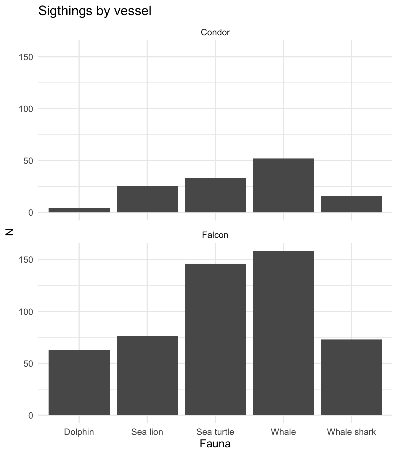
You are given a logbook of fauna sightings during whale watching tours from two vessels operating in the Revillagigedo Archipelago (A.K.A. the Socorro Islands), Mexico. You are about to embark on a tagging expedition, so you want to make sure you get on the right boat. Your goal is therefore to: a) Identify which vessel has the most sightings, and b) Identify the most frequent species sighted.
Post-it up
EVR 628 project folder. Save it into data/raw/.factors_dates_and_strings.R and save it into your scripts/01_processing/ foldertidyverse and janitor packages at the top of your scriptPost-it down
## SET UP ######################################################################
# Load packages ----------------------------------------------------------------
library(janitor)
library(tidyverse)Post-it up
tour_data <- and clean the column namestour_data_clean <- and add a new column called date that contains the date. We will build a large pipeline starting here.year, month, and day columns that we no longer needdate column all the way to the left# Load data -------------------------------------------------------------------
tour_data <- read_csv("data/raw/tour_data.csv") |>
clean_names()
dim(tour_data)
colnames(tour_data)
## PROCESSING ##################################################################
# Add a date -------------------------------------------------------------------
tour_data_clean <- tour_data |> # 3) New object
mutate(date = make_date(year, month, day)) |> # 4) Build my date
select(date, everything(), -c(year, month, day)) # 5) Remove and organize columns[1] 60 6[1] "year" "month" "day" "vessel" "passengers"
[6] "notes" The data look like this now:# A tibble: 6 × 4
date vessel passengers notes
<date> <chr> <dbl> <chr>
1 2025-01-01 Condor 21 8 Sea lions; 5 Whales; 4 Whale shark
2 2025-01-07 Falcon 6 5 whale; 7 Sea lions; 5 Sea turtle; 4 sea turtle
3 2025-01-13 Falcon 8 5 Dolphins
4 2025-01-19 Condor 6 4 Sea turtle; 4 sea turtle
5 2025-01-25 Condor 29 2 sea turtle; 8 whale
6 2025-02-01 Falcon 19 3 Whale shark; 7 whale Post-it down
Post-it up
separate_longer_delim() to create one row per species mentioned in the data## PROCESSING ##################################################################
# Add a date -------------------------------------------------------------------
tour_data_clean <- tour_data |>
mutate(date = make_date(year, month, day)) |>
select(date, everything(), -c(year, month, day)) |>
separate_longer_delim(cols = notes, delim = ";") |> # 1) Separate column into new rows
mutate(notes = str_to_lower(notes), # 2) All strings as lower case
notes = str_remove(notes, "s$")) # 3) All are singular now
cat("The data look like this now:")The data look like this now:head(tour_data_clean)# A tibble: 6 × 4
date vessel passengers notes
<date> <chr> <dbl> <chr>
1 2025-01-01 Condor 21 "8 sea lion"
2 2025-01-01 Condor 21 " 5 whale"
3 2025-01-01 Condor 21 " 4 whale shark"
4 2025-01-07 Falcon 6 "5 whale"
5 2025-01-07 Falcon 6 " 7 sea lion"
6 2025-01-07 Falcon 6 " 5 sea turtle" Post-it down
Post-it up
str_extract()pause to discuss
str_extract() function, build a new column called fauna that contains the species observed2fauna look right?str_extract() function, build a new column called n that contains the number of organisms observed (make sure it’s numeric)notes column## PROCESSING ##################################################################
# Add a date -------------------------------------------------------------------
tour_data_clean <- tour_data |>
mutate(date = make_date(year, month, day)) |>
select(date, everything(), -c(year, month, day)) |>
separate_longer_delim(cols = notes, delim = ";") |>
mutate(notes = str_to_lower(notes),
notes = str_remove(notes, "s$"),
fauna = str_extract(string = notes, pattern = "[a-z ]+$"), # 3) Extract fauna
fauna = str_squish(fauna), # 4) Remove white space
n = str_extract(string = notes, pattern = "[:digit:]+"), # 5) Extract n
n = as.numeric(n)) |> # and make sure it's numeric
select(-notes) # 6) Remove notes
cat("The data look like this now:")The data look like this now:head(tour_data_clean)# A tibble: 6 × 5
date vessel passengers fauna n
<date> <chr> <dbl> <chr> <dbl>
1 2025-01-01 Condor 21 sea lion 8
2 2025-01-01 Condor 21 whale 5
3 2025-01-01 Condor 21 whale shark 4
4 2025-01-07 Falcon 6 whale 5
5 2025-01-07 Falcon 6 sea lion 7
6 2025-01-07 Falcon 6 sea turtle 5Post-it down
Post-it up
tour_data_viz that contains the following columns3:vesselfaunan_per_tripPost-it down
## Build tour_data_viz ---------------------------------------------------------
tour_data_viz <- tour_data_clean |>
  group_by(vessel) |>
  mutate(effort = n_distinct(date)) |>
  group_by(vessel, fauna) |>
  summarize(n_per_trip = sum(n / effort),
            .groups = "drop")

cat("The data look like this now:")
The data look like this now:head(tour_data_viz)# A tibble: 6 × 3
vessel fauna n_per_trip
<chr> <chr> <dbl>
1 Condor dolphin 0.25
2 Condor sea lion 1.56
3 Condor sea turtle 2.06
4 Condor whale 3.25
5 Condor whale shark 1
6 Falcon dolphin 1.43## VISUALIZE ###################################################################
ggplot(data = tour_data_viz,
mapping = aes(x = str_to_sentence(fauna), # This is the only str-relevant change here
y = n_per_trip)) +
geom_col() +
facet_wrap(~vessel, ncol = 1) +
labs(title = "Sightings by vessel",
x = "Fauna",
y = "N") +
theme_minimal(base_size = 14)