Using `ggplot2`

Author

Juan Carlos Villaseñor-Derbez (JC)

Part 1: Build a basic plot

Open RStudio
Make sure you are in the EVR628 project
Create a new script, and save it to scripts as week2_ggplot.R
Add a basic descriptive header
Load packages

Code

library(EVR628tools)
library(tidyverse)

── Attaching core tidyverse packages ──────────────────────── tidyverse 2.0.0 ──
✔ dplyr     1.1.4     ✔ readr     2.1.5
✔ forcats   1.0.0     ✔ stringr   1.5.1
✔ ggplot2   3.5.2     ✔ tibble    3.3.0
✔ lubridate 1.9.4     ✔ tidyr     1.3.1
✔ purrr     1.1.0     
── Conflicts ────────────────────────────────────────── tidyverse_conflicts() ──
✖ dplyr::filter() masks stats::filter()
✖ dplyr::lag()    masks stats::lag()
ℹ Use the conflicted package (<http://conflicted.r-lib.org/>) to force all conflicts to become errors

Load data

Code

data(data_lionfish)

Inspect data

Code

glimpse(data_lionfish)

Rows: 109
Columns: 9
$ id              <chr> "001-Po-16/05/10", "002-Po-29/05/10", "003-Pd-29/05/10…
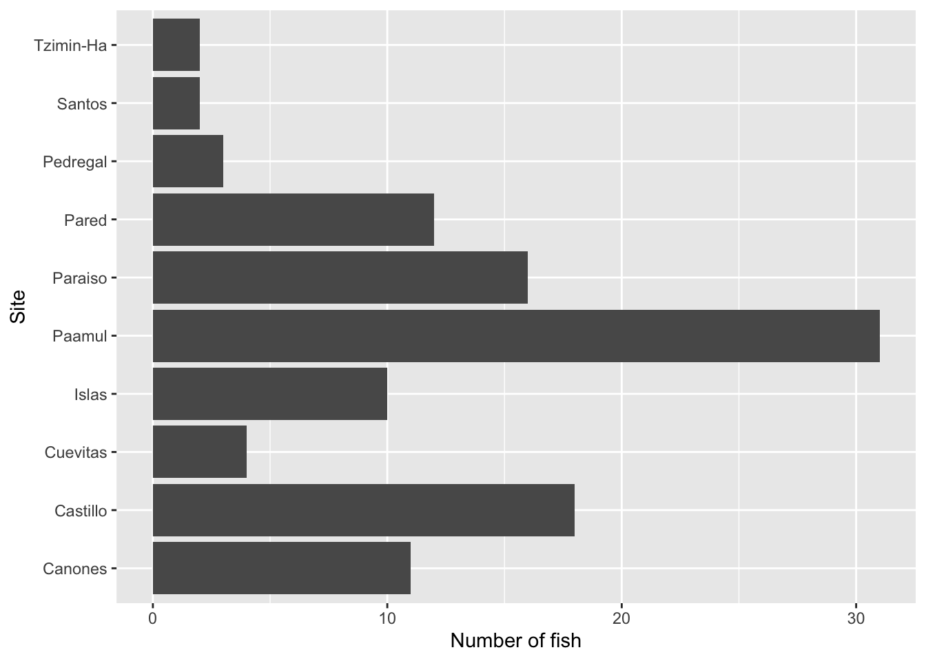
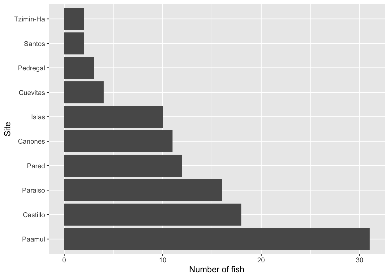
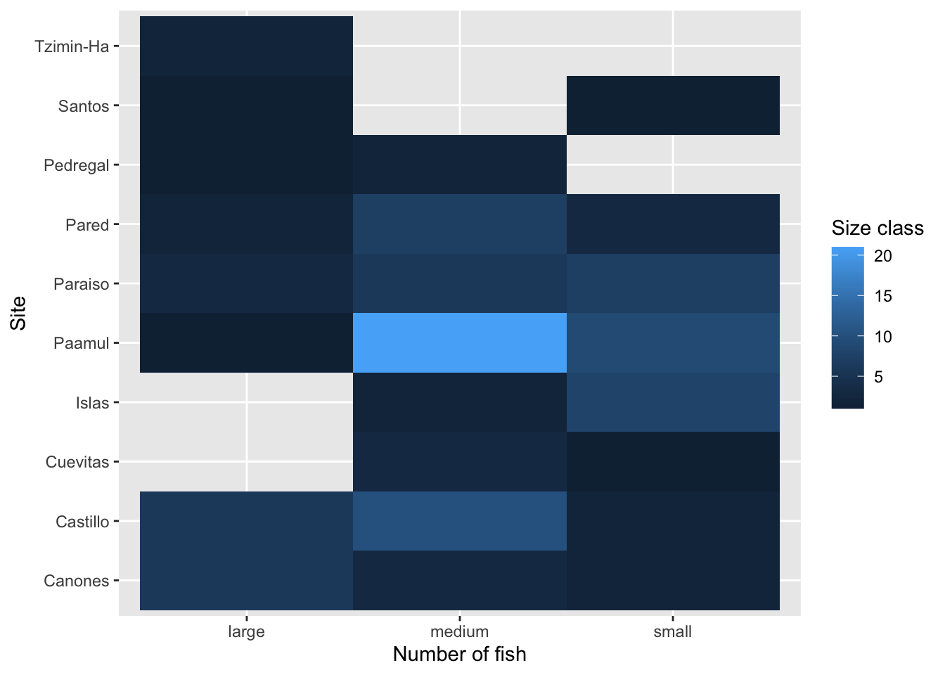
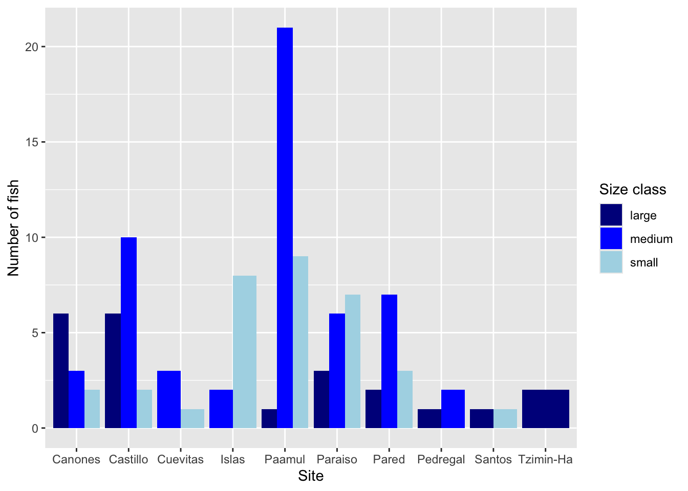
$ site            <chr> "Paraiso", "Paraiso", "Pared", "Canones", "Canones", "…
$ lat             <dbl> 20.48361, 20.48361, 20.50167, 20.47694, 20.47694, 20.5…
$ lon             <dbl> -87.22611, -87.22611, -87.21167, -87.23278, -87.23278,…
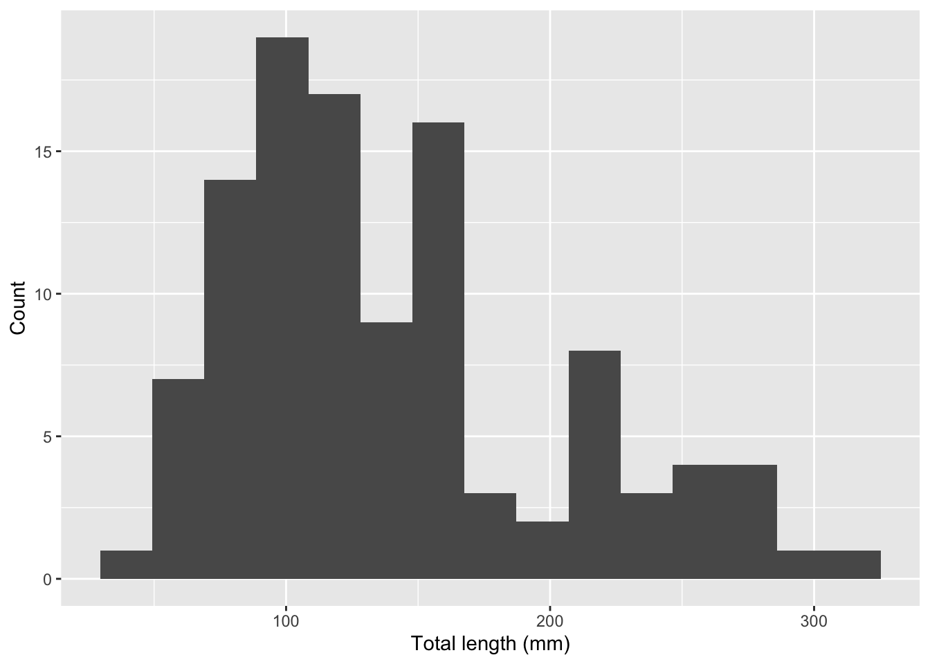
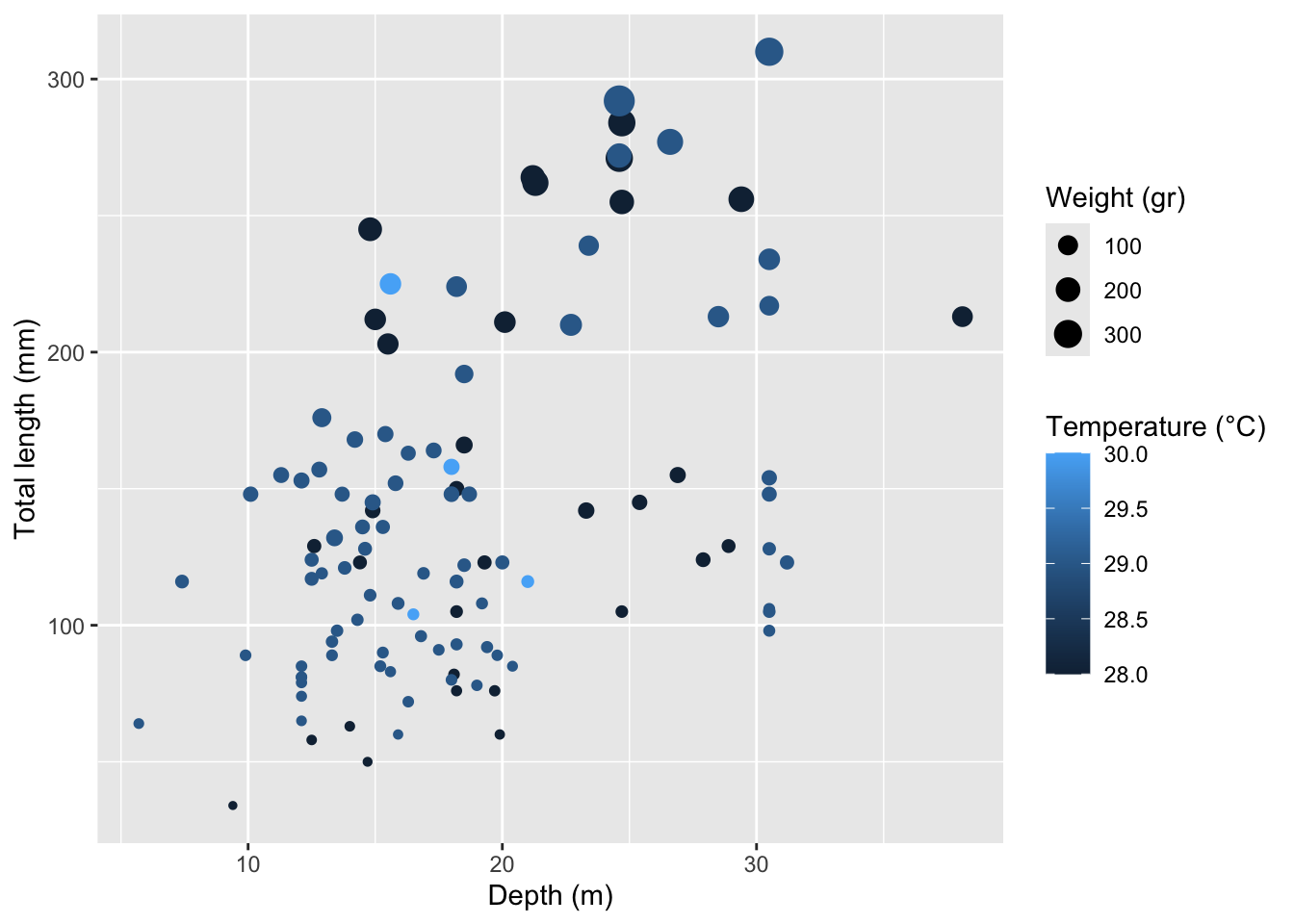
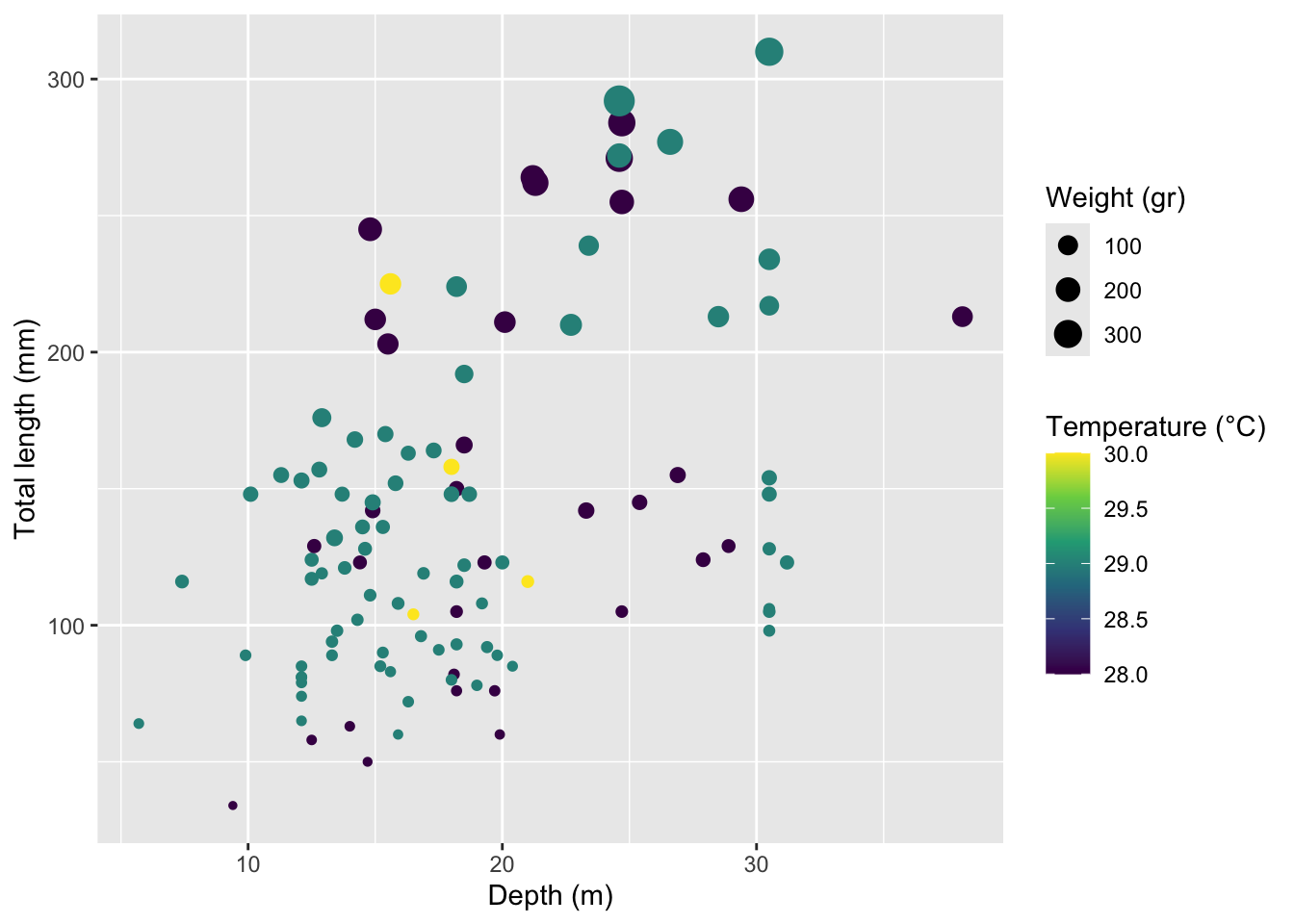
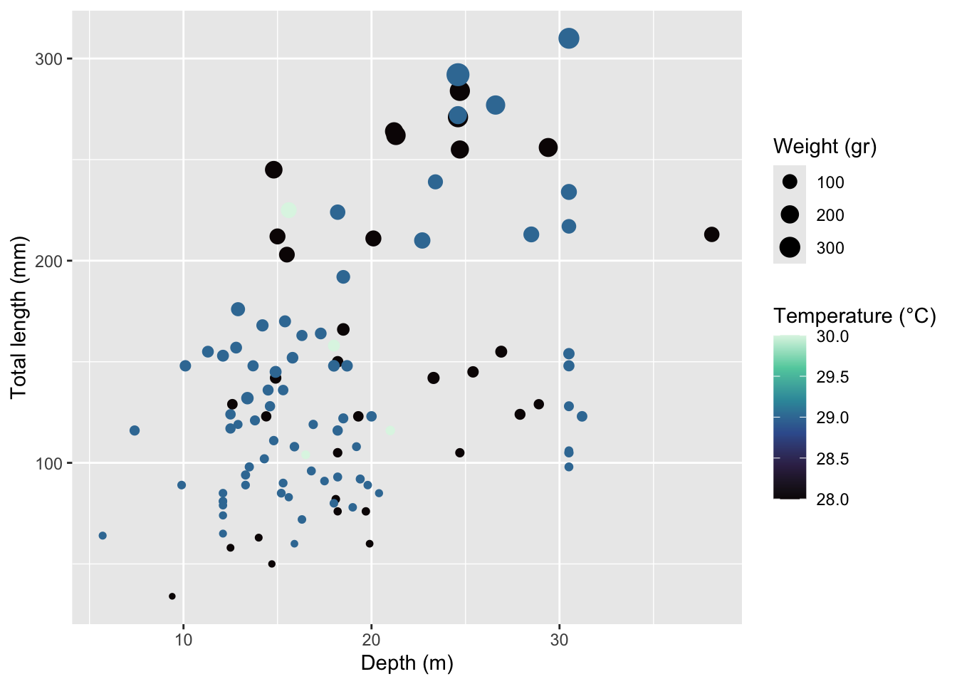
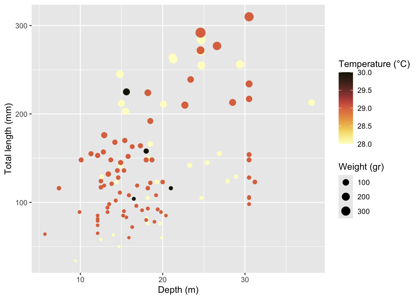
$ total_length_mm <dbl> 213, 124, 166, 203, 212, 210, 132, 122, 224, 117, 211,…
$ total_weight_gr <dbl> 112.70, 27.60, 52.30, 123.10, 129.00, 138.75, 50.29, 1…
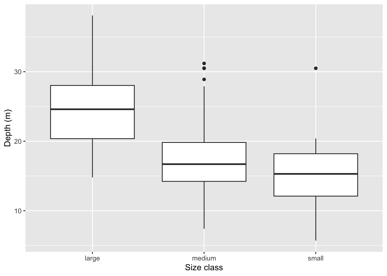
$ size_class      <chr> "large", "medium", "medium", "large", "large", "large"…
$ depth_m         <dbl> 38.1, 27.9, 18.5, 15.5, 15.0, 22.7, 13.4, 18.5, 18.2, …
$ temperature_C   <dbl> 28, 28, 28, 28, 28, 29, 29, 29, 29, 29, 28, 28, 28, 28…

The `ggplot` function

Show documentation: point out data and mapping
Specify data

Code

ggplot(data = data_lionfish)

The `aes` function

Show documentation
Explain a function inside a function
Then specify mapping
- Emphasis on use of commas and named arguments without quotations
Multiple lines and parentheses

Code

ggplot(data = data_lionfish,
       mapping = aes(x = depth_m, y = total_length_mm))

The `geom_point` function

Emphasiz on + for layering
Run with simple points
Show documentation and scroll down to the Aesthetics section
Show how to change colors / sizes etc…
Emphasize difference between using variables and constant values (inside vs outisde aes)

Code

ggplot(data = data_lionfish,
       mapping = aes(x = depth_m, y = total_length_mm)) +
  geom_point()

`labs` function

Code

ggplot(data = data_lionfish,
       mapping = aes(x = depth_m,
                     y = total_length_mm)) +
  geom_point(shape = 21,
             fill = "steelblue",
             size = 2) +
  labs(x = "Depth (m)",
       y = "Total weight (gr)",
       title = "Body length and depth",
       subtitle = "Larger fish tend to live deeper",
       caption = "Source EVR628tools::data_lionfish")

Part 2: Visualizing distributions

Distribution of a cateogrical variable

Categorical variable with geom_bar()
- basic with site
- with fct_infreq and site

Code

# Basic bar plot with site
ggplot(data = data_lionfish, aes(x = site)) +
  geom_bar() +
  coord_flip() +
  labs(x = "Site", y = "Number of fish")

Code

# Bar plot with sites ordered by frequency
ggplot(data = data_lionfish, aes(x = fct_infreq(site))) +
  geom_bar() +
  coord_flip() +
  labs(x = "Site", y = "Number of fish")

Distribution of a numeric variable

Numerical variable with geom_histogram()
- Distribution of lengths
- Show bins vs bin width
- \(k = 1 + 3.322 \times log_{10}(N)\)

Code

# Histogram of lengths
ggplot(data = data_lionfish, aes(x = total_length_mm)) +
  geom_histogram(bins = 15) +
  labs(x = "Total length (mm)", y = "Count")

Part 3: Visualizing relationships

A numerical and a categorical variable

depth by size class

Code

# Numerical vs categorical: depth by size class
ggplot(data = data_lionfish, aes(x = size_class, y = depth_m)) +
  geom_boxplot() +
  labs(x = "Size class", y = "Depth (m)")

Two categorical variables

N by size class and site

Code

# Two categorical variables: N by size class and site
ggplot(data = data_lionfish, aes(x = site, y = size_class)) +
  geom_bin2d() +
  coord_flip() +
  labs(x = "Site", y = "Number of fish", fill = "Size class")

Three or more

length vs depth with size for weight and color for temperature

Code

# Three or more variables: length vs depth with size for weight
ggplot(data = data_lionfish,
       aes(x = depth_m, y = total_length_mm, 
           size = total_weight_gr,
           color = temperature_C)) +
  geom_point() +
  scale_size_continuous(range = c(1, 5)) +
  labs(x = "Depth (m)", y = "Total length (mm)", 
       size = "Weight (gr)", color = "Temperature (°C)")

Part 4: Modifying colors

`scale__viridis_`

The easiest way is to use scale_*_viridis_*
- Check documentation
- An example

Code

p <- ggplot(data = data_lionfish,
       aes(x = depth_m, y = total_length_mm, 
           size = total_weight_gr,
           color = temperature_C)) +
  geom_point() +
  scale_size_continuous(range = c(1, 5)) +
  labs(x = "Depth (m)", y = "Total length (mm)", 
       size = "Weight (gr)", color = "Temperature (°C)") +
  scale_color_viridis_c()

p

viridis options

Show errors for wrong type of scale
Change to mako

Code

p + 
  scale_color_viridis_c(option = "mako")

Scale for colour is already present.
Adding another scale for colour, which will replace the existing scale.

`scale_color_gradientn`

scale_color_gradientn for continuous and custom palette
- Check documentation
- An example

Code

p +
  scale_color_gradientn(colours = palette_IPCC(var = "temp", type = "seq"))

Scale for colour is already present.
Adding another scale for colour, which will replace the existing scale.

`scale_color_gradient2`

scale_color_gradient vs scale_color_gradient2 for continuous / divergent with ends
- Check documentation
- An example

Code

# Green to orange
p +
  scale_color_gradient(low = "green",
                       high = "orange")

Scale for colour is already present.
Adding another scale for colour, which will replace the existing scale.

Code

# Going through white
p +
  scale_color_gradient2(low = "green",
                       mid = "white",
                       high = "orange")

Scale for colour is already present.
Adding another scale for colour, which will replace the existing scale.

Code

# Set white at 0
p +
  scale_color_gradient2(low = "green",
                       mid = "white",
                       high = "orange",
                       midpoint = 29)

Scale for colour is already present.
Adding another scale for colour, which will replace the existing scale.

scale_color_manual for discrete
- Check documentation
- An example

Code

p <- ggplot(data = data_milton,
            aes(x = iso_time, y = pressure, color = sshs)) +
  geom_point()

p

Code

p +
  scale_color_manual(values = palette_UM(n = 10))

Code

p + 
  scale_color_viridis_d()

scale_*_manual

Code

# Example with manual color scale for discrete variables
ggplot(data = data_lionfish, aes(x = site, fill = size_class)) +
  geom_bar(position = "dodge") +
  scale_fill_manual(values = c("small" = "lightblue", 
                               "medium" = "blue", 
                               "large" = "darkblue")) +
  labs(x = "Site", y = "Number of fish", fill = "Size class")

Helpful resources

ggplot cheatsheet

Part 5: Extra material if time allows

Saving plots

Repeat the entire process, one line at a time, showing how to save to an object
Then show how to save plot with ggsave
Show documentation of ggsave
Emphasize creating plot objects

Code

# Save plot to object
p <- ggplot(data = data_lionfish,
            mapping = aes(x = depth_m, y = total_length_mm)) +
  geom_point(shape = 21, fill = "steelblue", size = 2) +
  labs(x = "Depth (m)",
       y = "Total length (mm)",
       title = "Body length and depth")

Code

# Save plot to file
ggsave("lionfish_depth_length.png", p, width = 8, height = 6, dpi = 300)

Layering

Show data_milton documentation again
Build plot below
Show use of color vs fill inside main aes() (affecting line and points) vs aes() inside geom_point() (affecting only the poitns)

Code

p <- ggplot(data = data_milton,
            mapping = aes(x = iso_time,
                          y = pressure,
            )) +
  geom_line() +
  geom_point(aes(color = wind_speed),
             size = 2) 

p +
  scale_color_gradientn(colours = palette_IPCC(var = "wind", type = "seq"))

Facetting

Show documentation for facet_wrap and facet_grid
Show how each of these work

Code

# Facet wrap example
ggplot(data = data_lionfish, aes(x = depth_m, y = total_length_mm)) +
  geom_point() +
  facet_wrap(~size_class, ncol = 3) +
  labs(x = "Depth (m)", y = "Total length (mm)")

Code

# Facet grid example
ggplot(data = data_lionfish, aes(x = depth_m, y = total_length_mm)) +
  geom_point() +
  facet_grid(size_class ~ site) +
  labs(x = "Depth (m)", y = "Total length (mm)")

Code

# Facet wrap with different scales
ggplot(data = data_lionfish, aes(x = depth_m, y = total_length_mm)) +
  geom_point() +
  facet_wrap(~size_class, ncol = 3, scales = "free_y") +
  labs(x = "Depth (m)", y = "Total length (mm)")

Part 1: Build a basic plot

The ggplot function

The aes function

The geom_point function

labs function

Part 2: Visualizing distributions

Distribution of a cateogrical variable

Distribution of a numeric variable

Part 3: Visualizing relationships

A numerical and a categorical variable

Two categorical variables

Three or more

Part 4: Modifying colors

scale_*_viridis_*

viridis options

scale_color_gradientn

scale_color_gradient2

Helpful resources

Part 5: Extra material if time allows

Saving plots

Layering

Facetting

The `ggplot` function

The `aes` function

The `geom_point` function

`labs` function

`scale__viridis_`

`scale_color_gradientn`

`scale_color_gradient2`